nrow(data)  # number of rows
ncol(data)  # number of columns
dim(data) # dimensions: rows & columnsR Tips
R
TidyR
CSS Color
Snippets
Common R tips & code snippets: dplyr data manipulation, stringr text operations, CSS color names, code cheatsheets, etc.
Top Tips
| Tip | Notes |
|---|---|
| Relative Paths | Keep data and code in the same folder; use relative paths to avoid errors caused by spaces in paths |
Add na.rm = TRUE to stats |
Required for sum, mean, sd, IQR, etc.; otherwise returns NA when missing values exist |
| Clarify unit of observation | Confirm what each row represents; for mixed types (e.g. post/comment), filter first: filter(type == "post") |
Name computed columns inside count() |
e.g. count(month = month(date)) |
Distinguish filter() from select() |
filter(condition) filters rows; select(col) selects columns (filter operators) |
Use nrow() / pull() to extract values |
nrow() returns row count; pull() extracts a single value from a data frame |
| Use stringr + Regex for text | str_length() counts characters; str_count(text, "\\S+") counts words |
| Reassign after adding columns | data <- data |> mutate(…) |
TRUE / FALSE aliases |
Equivalent to T / F |
| Use RStudio Snippets | Use code templates to reduce repetitive typing |
1 Exploring Data
1.1 Dimensions
1.2 Filtering
Filter: Count observations (rows) matching a condition
data |> filter(condition) |> nrow()# Example: data has a type column with only "comment" and "post" values
# How many posts are there in total?
# Method 1: nrow() directly returns the row count; other dplyr functions require pull() to extract the value
data |>
filter(type == "post") |>
nrow()
# Method 2:
data |>
filter(type == "post") |>
count(type) |> # swapping count and filter order gives the same result
pull(n)
# Method 3:
data |>
filter(type == "post") |>
summarize(n = n()) |>
pull(n)1.3 Most Frequent Category
data |> count(col, sort=T) |> head(1) |> pull(col)# Example: data has a date column with Date datatype (yyyy-mm-dd)
# Which year had the most posts?
# Method 1:
data |>
filter(type == "post") |>
count(year = year(date), sort = TRUE) |>
head(1) |> # sort=T was specified above, so head(1) works directly
pull(year)
# Method 2:
data |>
filter(type == "post") |>
count(year = year(date)) |> # count produces a two-column df: year and n
slice_max(n, n = 1) |> # first n is the column name, second is row count — selects the row with max n
pull(year)1.4 Min/Max Value
Min/Max value of a column
# When asking about all rows (e.g. "overall activity", "across the whole dataframe")
# No need for pipe; if there's a condition (e.g. "only posts"), filter first
min(data$col, na.rm = TRUE)
max(data$col, na.rm = TRUE)
1.5 Unique Values
Unique values of a column
n_distinct(data$col)  # unique value count
unique(data$col)      # unique values
2 Cleaning Data
2.1 Rounded Mean or Median
summarize(mean = round(mean(col, na.rm = TRUE), 2)) |> pull(mean)# Example: mean score of posts in 2019, rounded to 2 decimal places
data |>
filter(type == "post" & year(date) == 2019) |>
summarize(mean = round(mean(score, na.rm = TRUE), 2)) |>
pull(mean)# Example: median score per year, rounded to 2 decimal places,
# sorted by median score descending, returned as a dataframe
data |>
filter(type == "post") |>
group_by(year = year(date)) |>
summarize(
median_score = round(median(score, na.rm = TRUE), 2),
.groups = "drop" # group + summarize requires .groups = "drop"
) |>
arrange(desc(median_score)) # sort descending; can also write arrange(-median_score)2.2 Add a Column
data <- data |> mutate(new_col = operation_on_col)# Add a character count column
data <- data |>
mutate(text_length = str_length(text))
# Add a word count column
data <- data |>
mutate(word_count = str_count(text, "\\S+"))2.3 Value at Row Maximum
data |>
slice_max(col1, n = 1) |>
pull(col2)# Example: who is the author of the post with the highest word_count?
data |>
# we want posts only, but data contains other types — filter first
filter(type == "post") |>
slice_max(word_count, n = 1) |>
pull(author)2.4 Text Length
str_length(text)2.5 Word Count
str_count(text, "\\S+")3 Visualization
3.1 Bar Chart
# Example: bar chart of monthly post count in 2019
# Step 1: prepare data for plotting
bar_data <- data |>
filter(type == "post" & year(date) == 2019) |>
count(month = month(date)) # no need for sort = TRUE
# Step 2: plot
ggplot(bar_data, aes(x = factor(month), y = n)) +
# month is numeric; using it directly makes the x-axis continuous — use factor(month)
# Note: months are ordered in time, so no need to sort bars by size;
# for nominal vars like "region", use x = reorder(area, -n) for descending order
# if there are many regions or long names, use coord_flip() for a horizontal bar chart
# Use geom_col (not _bar): y is a pre-computed value from the n column,
# not asking ggplot to count rows per category on the fly
geom_col(fill = "steelblue") + # choose any color you like
labs(
title = "Monthly Post Count in 2019",
x = "Month",
y = "Post Count"
)3.2 Histogram
# Plot histogram of post scores
ggplot(data |> filter(type == "post"), aes(x = score)) +
geom_histogram(fill = "steelblue", bins = 30) + # set number of bins
labs(
title = "Post Score Distribution",
x = "Post Score",
y = "Frequency"
)4 Text Analysis
# Example: show top 10 most frequent words in posts as a dataframe, and save the top word as a variable
data |>
filter(type == "post") |>
unnest_tokens(word, text) |>
anti_join(stop_words) |>
count(word, sort = TRUE) |>
head(10)
top1 <- data |>
filter(type == "post") |>
unnest_tokens(word, text) |>
anti_join(stop_words) |>
count(word, sort = TRUE) |>
head(1) |>
pull(word)5 Statistics
5.1 Compute Statistics
round(sd(data$col, na.rm = TRUE), 2)
IQR(data$col, na.rm = TRUE)5.2 Filter Before Computing
filter(condition) |> summarize(mean = mean(col, na.rm = TRUE)) |> pull(mean)5.3 Statistical Test + Interpret Results
t.test(col1 ~ col2, data = data)5.4 Linear Regression + Coefficients
m <- lm(col1 ~ col2, data = data)
coef(m)[[1]] # intercept
coef(m)[[2]] # slope6 More Tips
6.1 Common dplyr Functions
| Function | Purpose | Example |
|---|---|---|
filter(condition) |
Keep rows matching the condition | filter(type == "post" & score > 10) |
select(col) |
Select columns by name | select(col1), col1:col3, -col3 |
count(col) |
Count rows per unique value in this column | count(year = year(date), sort = TRUE) |
nrow() |
Count current rows | Takes no arguments; typically used with filter():filter(score > mean(score, na.rm=T)) |> nrow() |
slice_max(col, n=rows) |
Select the row(s) with the maximum value | slice_max(score, n = 10) |
pull(col) |
Return the value(s) of this column | Typically narrow down to one row with filter / slice_max / head / summarize, then pull(col), e.g.:summarize(mean_age=mean(age,na.rm=T))|> pull(mean_age) |
mutate(new_col=expr) |
Add/modify columns in place | mutate(perc = col1/col2*100) |
group_by(col) |
Group (used with summarize/mutate) | group_by(age) |
summarize(...) |
Return a summary | group_by(age) |>summarize(avg = mean(score, na.rm=T), .groups=“drop”) |
arrange(col) |
Sort (ascending by default) | arrange(age, desc(score)) |
glimpse(df) |
Inspect structure (≈ str()) |
glimpse(data) |
rename(new=old) |
Rename columns (does not create new columns) | rename(new_col = old_col) |
group_by+summarize: must add.groups="drop"; keeps grouping and summary columns, compressing rows to one per groupgroup_by+mutate: keeps all columns with row count unchanged; must callungroup()afterwardmean(condition)→ proportion satisfying the condition;sum(condition)→ count satisfying the condition
Note the difference between
nrow()andn(): both count rows, butnrow()takes a data frame as argument;n()is a dplyr context function only usable insidesummarize()/mutate()(e.g.summarize(number_of_observation = n())); usenrow()in a pipe
# Example:
# data has a type column with only "post" and "comment" values;
# another column word_count is the word count of each post/comment
# How many posts have fewer than 10 words?
data |>
filter(type == "post" & word_count < 10) |>
nrow() # directly returns a number
data |>
filter(type == "post" & word_count < 10) |>
summarize(count = n()) |> # summarize() still returns a dataframe
pull(count) # pull is needed to get the scalar value6.2 Logical Operators in filter()
| Operator | Description |
|---|---|
! & | |
not / and / or |
== != |
vector equality / inequality |
> >= < <= |
greater than / ≥ / less than / ≤ |
%in% |
whether the left element exists in the right vector (not element-wise comparison) |
%in%checks element membership;==matches by position (recycled when lengths differ)
# Example:
# data has a date column with Date datatype (yyyy-mm-dd);
# another column type has "post" and "comment" values;
# How many posts have year 2019 or 2023?
data |>
filter(type == "post" & year(date) %in% c(2019, 2023)) |>
nrow()
# 1. Condition 1: type is "post", use ==
# 2. Condition 2: year is 2019 or 2023,
# first extract the year from date using year() which gets the year from a full date (yyyy-mm-dd);
# then two options to match 2019 or 2023:
# 1) (year(date) == 2019 | year(date) == 2023)
# 2) year(date) %in% c(2019, 2023)
# 3. Both conditions must be met, combine with &
# Note: if you use option 1), wrap it in parentheses before combining with &
# 4. Use nrow() to count rows matching the filter condition
# Extension:
# To count all posts from 2019 through 2023, use:
# year(date) %in% 2019:2023
# because 2019:2023 expands to c(2019, 2020, 2021, 2022, 2023)6.3 Helper Functions in select()
Note: select() picks columns; filter() picks rows — they are not interchangeable
| Syntax | Effect |
|---|---|
select(col1:col3) |
Select col1 through col3 |
select(-col3) |
Exclude col3 |
select(contains(“x”)) |
Column name contains “x” |
select(starts_with(“c”)) |
Column name starts with “c” |
select(ends_with(“3”)) |
Column name ends with “3” |
select(everything()) |
Select all columns |
6.4 Regex
# Add a character count column
data <- data |>
    mutate(text_length = str_length(text))

# Add a word count column
data <- data |>
mutate(word_count = str_count(text, "\\S+"))| Pattern | Meaning | Example | Matches |
|---|---|---|---|
. |
any single character | "a.c" |
“abc”, “a1c”, “a c” |
^ |
start of string | "^The" |
“The dog” but not “See The dog” |
$ |
end of string | "end$" |
“the end” but not “endless” |
* |
preceding character zero or more times | "ab*c" |
“ac”, “abc”, “abbc” |
+ |
preceding character one or more times | "ab+c" |
“abc”, “abbc” but not “ac” |
? |
preceding character zero or one times | "colou?r" |
“color”, “colour” |
\\ |
escape special character | "\\." |
literal period “.” |
| Pattern | Meaning | Example |
|---|---|---|
[abc] |
matches a, b, or c | "[aeiou]" matches vowels |
[a-z] |
any lowercase letter | |
[A-Z] |
any uppercase letter | |
[0-9] |
any digit | equivalent to \\d |
[^abc] |
any character except a, b, c | [^0-9] matches non-digits |
| Shorthand | Meaning | Equivalent |
|---|---|---|
\\d |
any digit | [0-9] |
\\D |
any non-digit | [^0-9] |
\\w |
any word character | [a-zA-Z0-9_] |
\\W |
any non-word character | [^a-zA-Z0-9_] |
\\s |
any whitespace character | space, tab, newline |
\\S |
any non-whitespace character |
6.5 stringr Functions
| Function | Purpose | Example |
|---|---|---|
str_detect() |
whether a match exists (TRUE/FALSE) | str_detect(x, "pattern") |
str_subset() |
return matching elements | str_subset(x, "pattern") |
str_extract() |
extract first match | str_extract(x, "pattern") |
str_extract_all() |
extract all matches | str_extract_all(x, "pattern") |
str_replace() |
replace first match | str_replace(x, "pattern", "replacement") |
str_replace_all() |
replace all matches | str_replace_all(x, "pattern", "replacement") |
str_match() |
extract capture groups from first match | str_match(x, "pattern") |
str_count() |
count number of matches | str_count(x, "pattern") |
str_split() |
split string by pattern | str_split(x, "pattern") |
6.6 Common Color Names
| Color Name | Preview | Color Name | Preview |
|---|---|---|---|
| pink | ████ | beige | ████ |
| lightpink | ████ | darkseagreen | ████ |
| lightcoral | ████ | mediumseagreen | ████ |
| palevioletred | ████ | forestgreen | ████ |
| rosybrown | ████ | green | ████ |
| indianred | ████ | seagreen | ████ |
| firebrick | ████ | teal | ████ |
| tomato | ████ | lightseagreen | ████ |
| coral | ████ | mediumaquamarine | ████ |
| salmon | ████ | powderblue | ████ |
| lightsalmon | ████ | lightblue | ████ |
| sandybrown | ████ | skyblue | ████ |
| orange | ████ | lightskyblue | ████ |
| peru | ████ | lightsteelblue | ████ |
| tan | ████ | steelblue | ████ |
| wheat | ████ | mediumpurple | ████ |
| bisque | ████ | plum | ████ |
| linen | ████ | thistle | ████ |
6.7 Relative Paths
Relative path. Place your Rmd file and CSV in the same folder; read with read_csv("./exam-data.csv") — ./ means the current folder. Relative paths are recommended to avoid errors caused by spaces in absolute paths.
Absolute path. In Finder, select the file and press ⌥⌘C to copy the absolute path, e.g. data <- read_csv("/Users/username/EM747/mid-exam/exam-data.csv").
6.8 RStudio Snippet
In RStudio > Tools > Edit Code Snippets
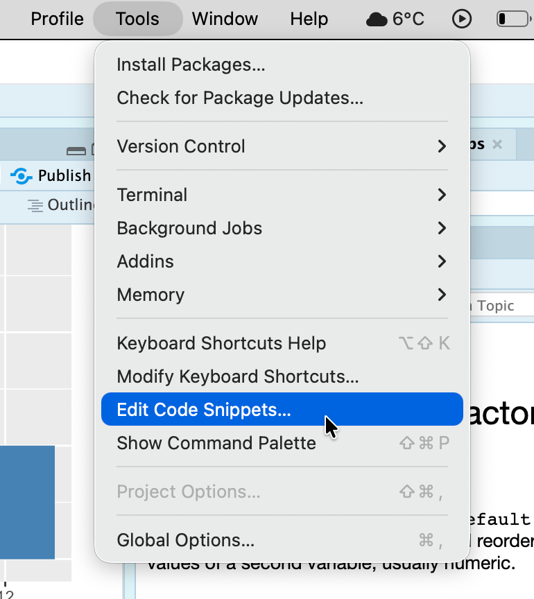
R > scroll to the bottom and add new code > Save
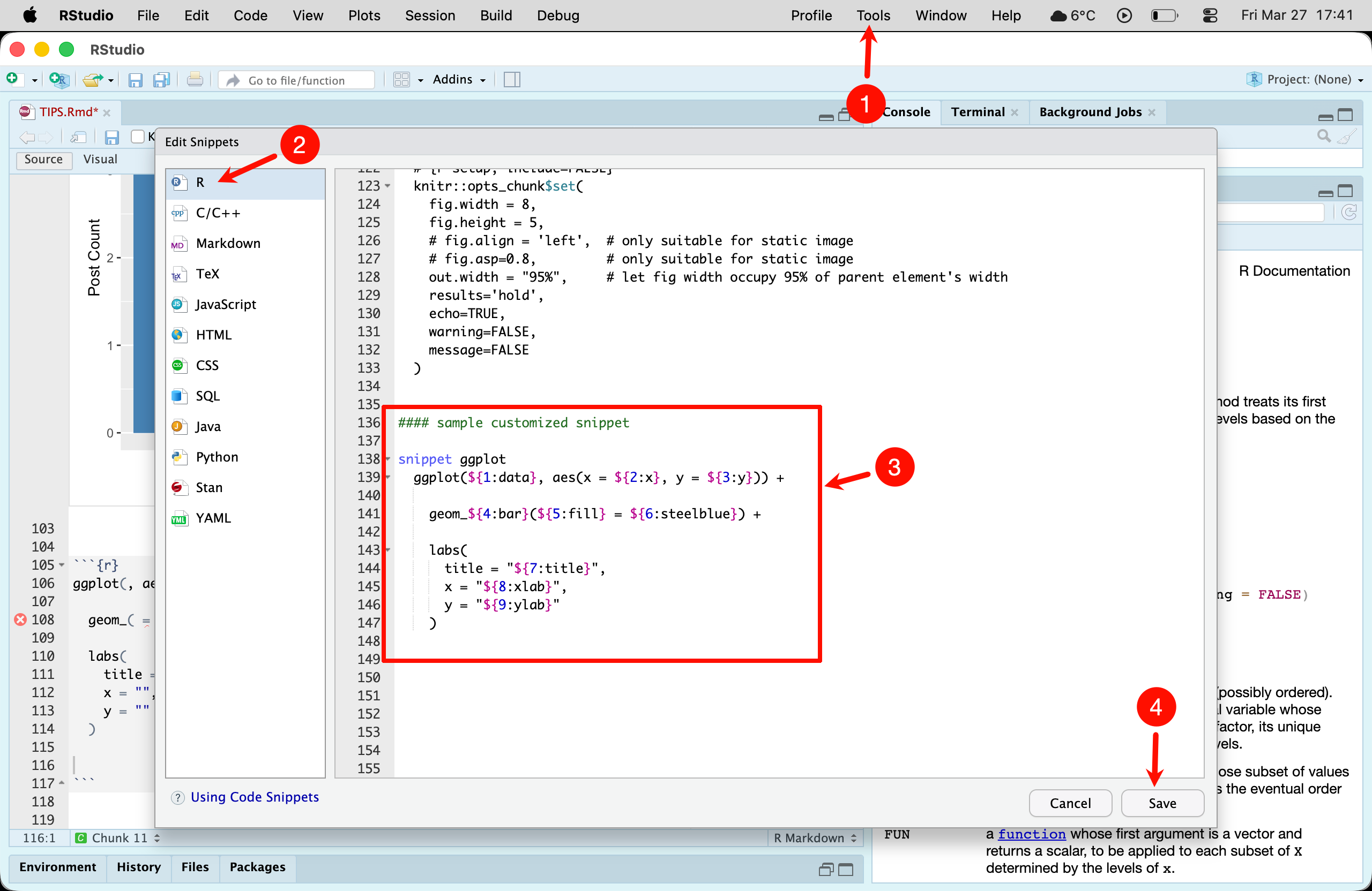
For example, a ggplot template:
snippet ggplot
    ggplot(${1:data}, aes(x = ${2:x}, y = ${3:y})) +
        geom_${4:bar}(${5:fill} = "${6:steelblue}") +
        labs(
            title = "${7:title}",
            x = "${8:xlab}",
            y = "${9:ylab}"
        )
After saving, type ggplot in an R code block and select the snippet:
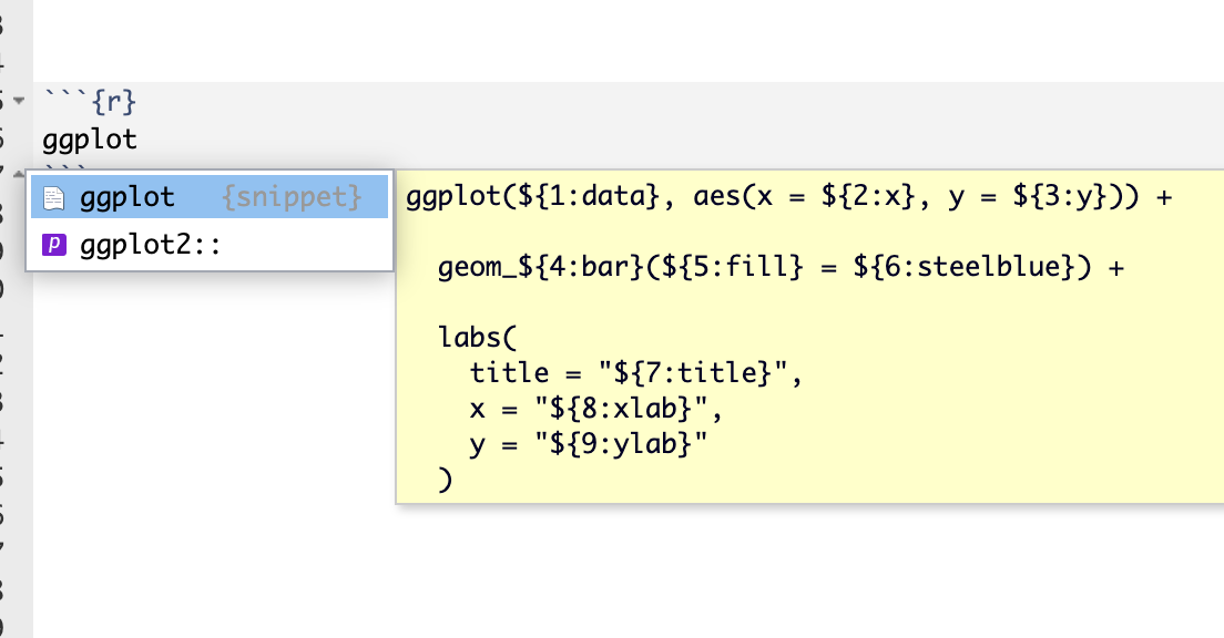
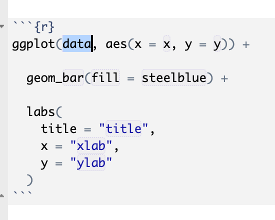
Press Enter and the template is inserted automatically: