Environment and Versions
python==3.12
pandas==2.2.2
matplotlib==3.9.x
seaborn==0.13.2python==3.12
pandas==2.2.2
matplotlib==3.9.x
seaborn==0.13.2Note: If you are using a local environment such as Jupyter or VS Code, install Seaborn first. If you are using Google Colab, Seaborn is already available and does not need to be installed manually.
pip install seabornimport seaborn as sns
import matplotlib.pyplot as pltmatplotlib.pyplot is usually abbreviated as plt so plotting functions can be called more conveniently. Using the full path is not recommended:
import matplotlib.pyplot
matplotlib.pyplot.plot(...)
matplotlib.pyplot.show()
Recommended style:
import matplotlib.pyplot as plt  # Import with the alias 'plt' for later use
plt.plot(...)
plt.show()mpl: an alias for matplotlib, commonly used for global configuration, lower-level properties, and advanced submodules such as colormaps and 3D plotting.plt: an alias for matplotlib.pyplot, the main everyday interface for quickly creating and managing figures.Reference: matplotlib.pyplot tutorial
df = sns.load_dataset('penguins')  # Load the penguins example dataset
df.info()  # View column names, data types, and non-null counts
<class 'pandas.core.frame.DataFrame'>
RangeIndex: 344 entries, 0 to 343
Data columns (total 7 columns):
# Column Non-Null Count Dtype
--- ------ -------------- -----
0 species 344 non-null object
1 island 344 non-null object
2 bill_length_mm 342 non-null float64
3 bill_depth_mm 342 non-null float64
4 flipper_length_mm 342 non-null float64
5 body_mass_g 342 non-null float64
6 sex 333 non-null object
dtypes: float64(4), object(3)
memory usage: 18.9+ KBFloat Data
Floating-point columns such as length and mass are continuous numerical variables. Variables with a true zero, where 0 means “none”, are ratio data, such as length and mass. Variables without a true zero are interval data, such as temperature.
Object Data
Species names and island names are nominal data. Sex is ordinal data.
df.head() # View the first five rows| species | island | bill_length_mm | bill_depth_mm | flipper_length_mm | body_mass_g | sex | |
|---|---|---|---|---|---|---|---|
| 0 | Adelie | Torgersen | 39.1 | 18.7 | 181.0 | 3750.0 | Male |
| 1 | Adelie | Torgersen | 39.5 | 17.4 | 186.0 | 3800.0 | Female |
| 2 | Adelie | Torgersen | 40.3 | 18.0 | 195.0 | 3250.0 | Female |
| 3 | Adelie | Torgersen | NaN | NaN | NaN | NaN | NaN |
| 4 | Adelie | Torgersen | 36.7 | 19.3 | 193.0 | 3450.0 | Female |
df.tail() # View the last five rows| species | island | bill_length_mm | bill_depth_mm | flipper_length_mm | body_mass_g | sex | |
|---|---|---|---|---|---|---|---|
| 339 | Gentoo | Biscoe | NaN | NaN | NaN | NaN | NaN |
| 340 | Gentoo | Biscoe | 46.8 | 14.3 | 215.0 | 4850.0 | Female |
| 341 | Gentoo | Biscoe | 50.4 | 15.7 | 222.0 | 5750.0 | Male |
| 342 | Gentoo | Biscoe | 45.2 | 14.8 | 212.0 | 5200.0 | Female |
| 343 | Gentoo | Biscoe | 49.9 | 16.1 | 213.0 | 5400.0 | Male |
df.sample(5) # Randomly sample five rows| species | island | bill_length_mm | bill_depth_mm | flipper_length_mm | body_mass_g | sex | |
|---|---|---|---|---|---|---|---|
| 123 | Adelie | Torgersen | 41.4 | 18.5 | 202.0 | 3875.0 | Male |
| 166 | Chinstrap | Dream | 45.9 | 17.1 | 190.0 | 3575.0 | Female |
| 240 | Gentoo | Biscoe | 50.2 | 14.3 | 218.0 | 5700.0 | Male |
| 7 | Adelie | Torgersen | 39.2 | 19.6 | 195.0 | 4675.0 | Male |
| 19 | Adelie | Torgersen | 46.0 | 21.5 | 194.0 | 4200.0 | Male |
Note: Function vs. Method
df.info(), df.head(), df.tail(), and df.sample() are all methods of a DataFrame object. They must be called from a specific object and cannot be used independently.
pd.read_csv() is a predefined Pandas function and can be called directly:
df = pd.read_csv('file_path')By contrast, df.sample() is a method that operates on the df object:
df.sample(4)| species | island | bill_length_mm | bill_depth_mm | flipper_length_mm | body_mass_g | sex | |
|---|---|---|---|---|---|---|---|
| 227 | Gentoo | Biscoe | 46.7 | 15.3 | 219.0 | 5200.0 | Male |
| 120 | Adelie | Torgersen | 36.2 | 17.2 | 187.0 | 3150.0 | Female |
| 272 | Gentoo | Biscoe | 45.1 | 14.4 | 210.0 | 4400.0 | Female |
| 62 | Adelie | Biscoe | 37.6 | 17.0 | 185.0 | 3600.0 | Female |
# Basic bar plot: the x-axis is categorical, and the y-axis shows the mean by default.
# The black error bars show 95% confidence intervals.
sns.barplot(data=df, x='island', y='body_mass_g')
plt.show()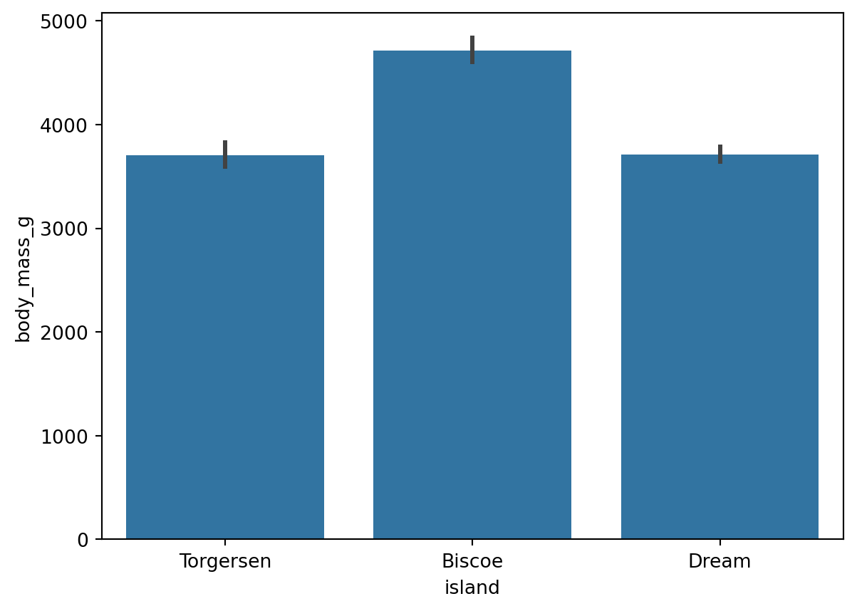
# estimator='sum': use the sum as the bar height instead of the default mean
sns.barplot(data=df, x='island', y='body_mass_g', estimator='sum')
plt.show()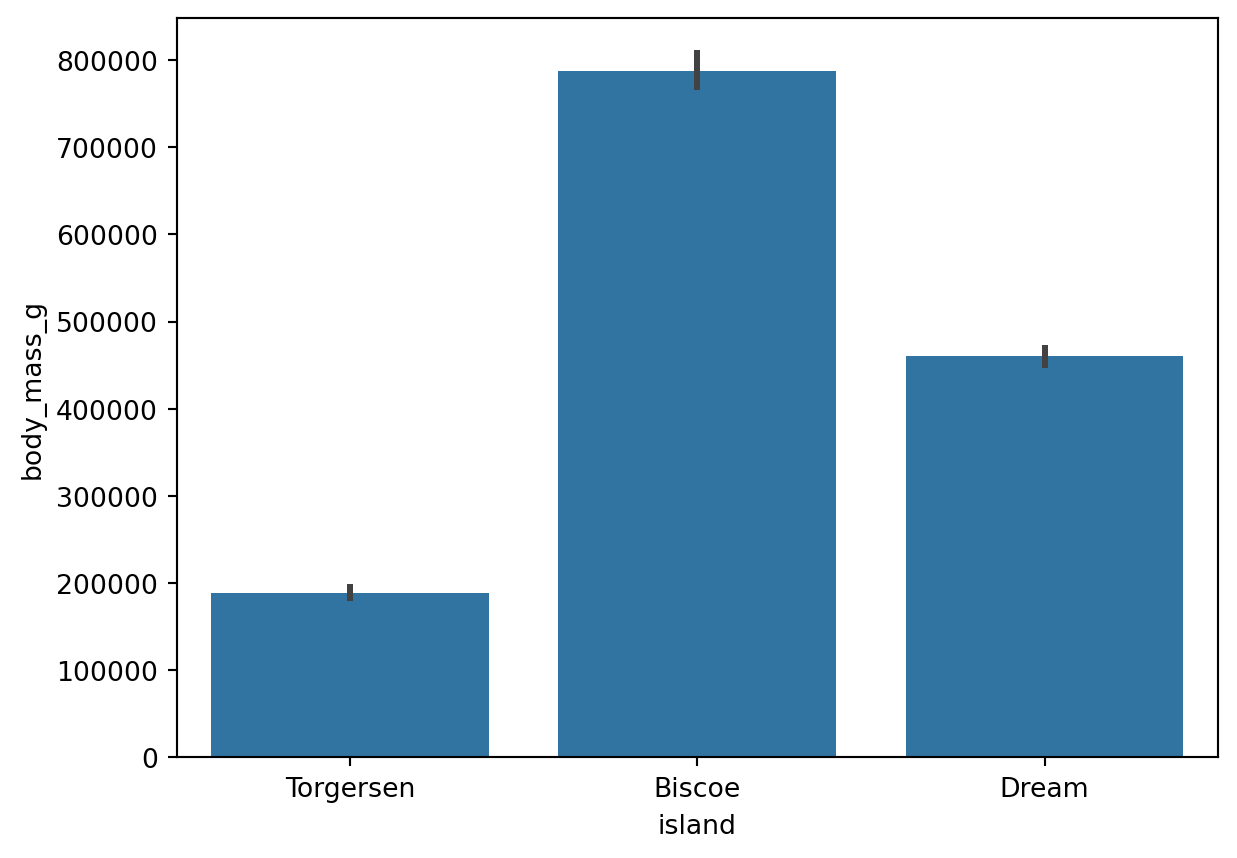
Reference: sns.barplot() documentation (estimator parameter)
sns.__version__ # View the current Seaborn version. Since 0.13, the default is a single color to avoid meaningless color distinctions.'0.13.2'# Check: the mean body mass for Biscoe Island is the bar height shown in the chart.
df.loc[df['island'] == 'Biscoe', 'body_mass_g'].mean()4716.017964071856# Count plot: automatically counts the number of observations in each category
sns.countplot(data=df, x='species')
plt.show()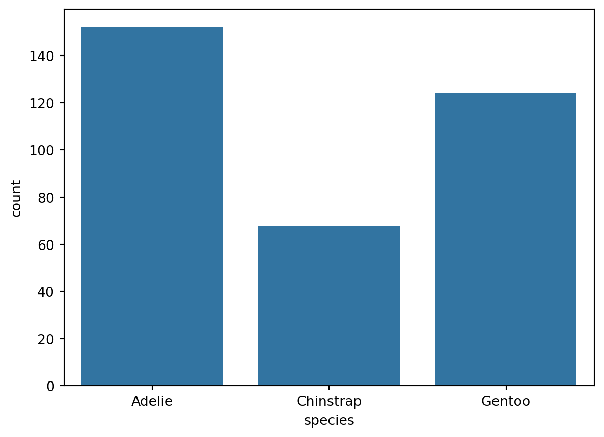
Reference: sns.countplot() documentation
Use the hue parameter to group by category, and set errorbar=None to remove error bars.
# Group by sex with hue, and remove error bars with errorbar=None
sns.barplot(data=df, x='island', y='body_mass_g', errorbar=None, hue='sex')
plt.show()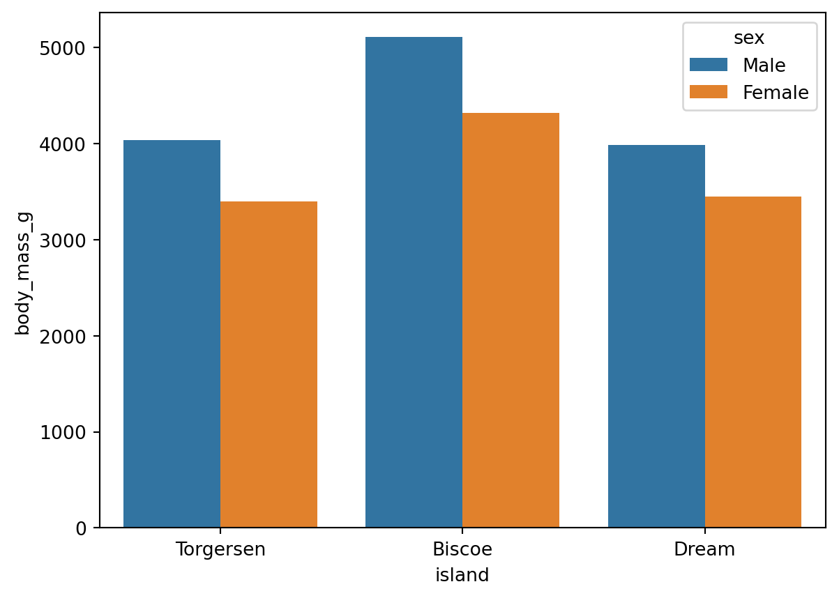
Reference: sns.barplot() documentation (errorbar and hue parameters)
When x-axis labels are too long, use plt.xticks() to rotate them:
sns.barplot(data=df, x='island', y='body_mass_g', errorbar=None, hue='sex')

# Rotate labels by 45 degrees. ha='right' aligns the right edge of each label with the tick.
plt.xticks(rotation=45, ha='right')
plt.show()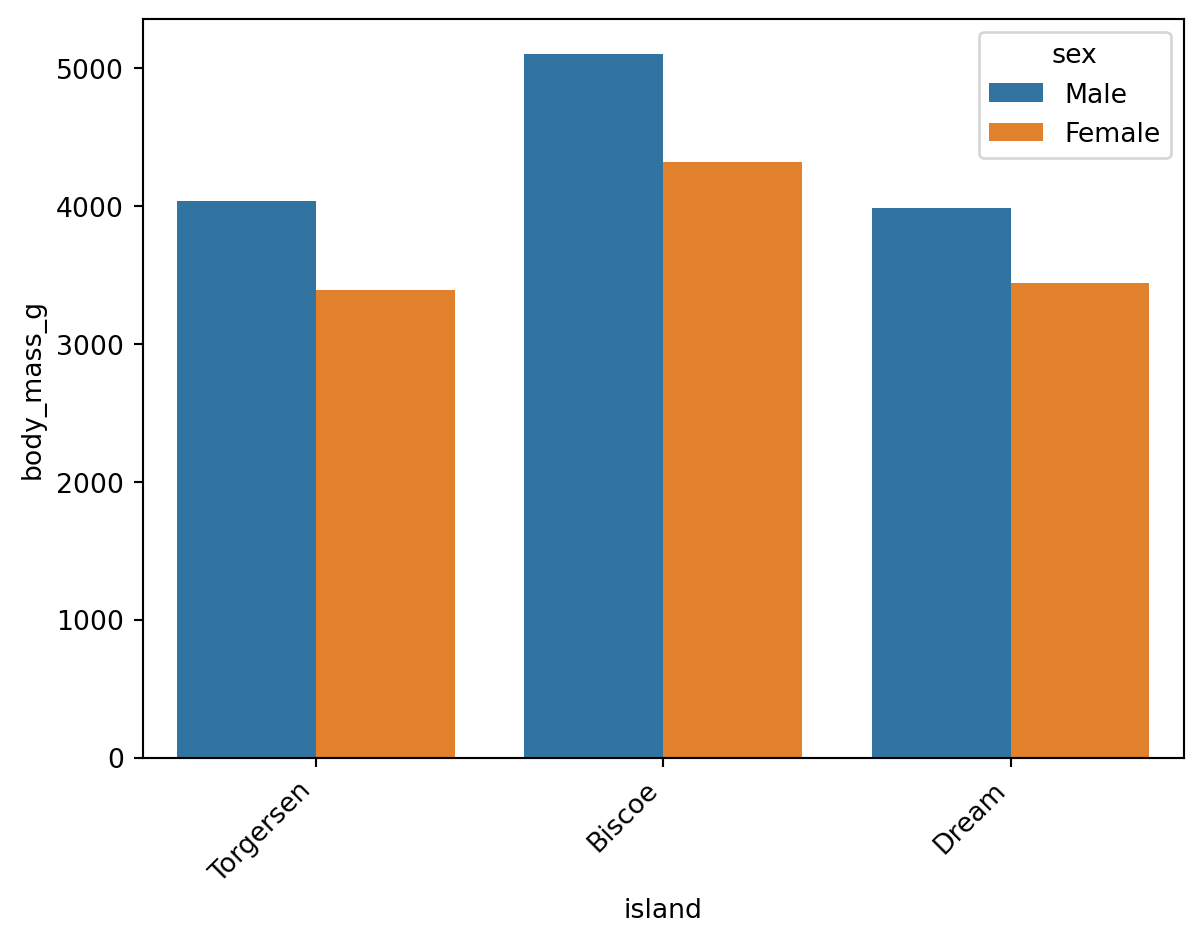
Reference: plt.xticks() documentation (kwargs section)
Wilke (2019, chap. 6.1) suggests that when labels are dense, a horizontal layout is easier to read than rotated labels:
# Swap the x and y axes: a horizontal layout is easier to read when labels are dense.
sns.barplot(data=df, y='island', x='body_mass_g', errorbar=None, hue='sex')
plt.show()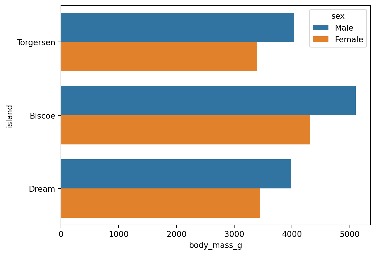
The same idea applies to count plots:
sns.countplot(data=df, y='species', hue='sex')
plt.show()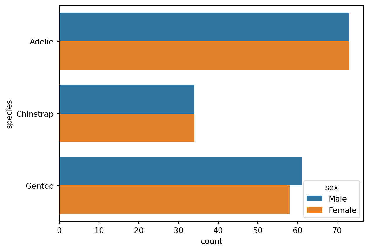
# Set the global plotting theme. It applies to all subsequent Seaborn charts.
# Use sns.reset_orig() to restore the default theme.
sns.set_theme(font_scale=1.2, style='darkgrid')
sns.set_theme() sets the global plotting theme for all later Seaborn charts. Call sns.reset_orig() to restore the default theme.
# Define a chart object named ax
ax = sns.barplot(
    data=df, x='body_mass_g', y='island',
    errorbar=None, hue='sex',
)

# Set the title and axis labels
ax.set(title='Penguin', xlabel='Body Mass (g)', ylabel='Island')
plt.show()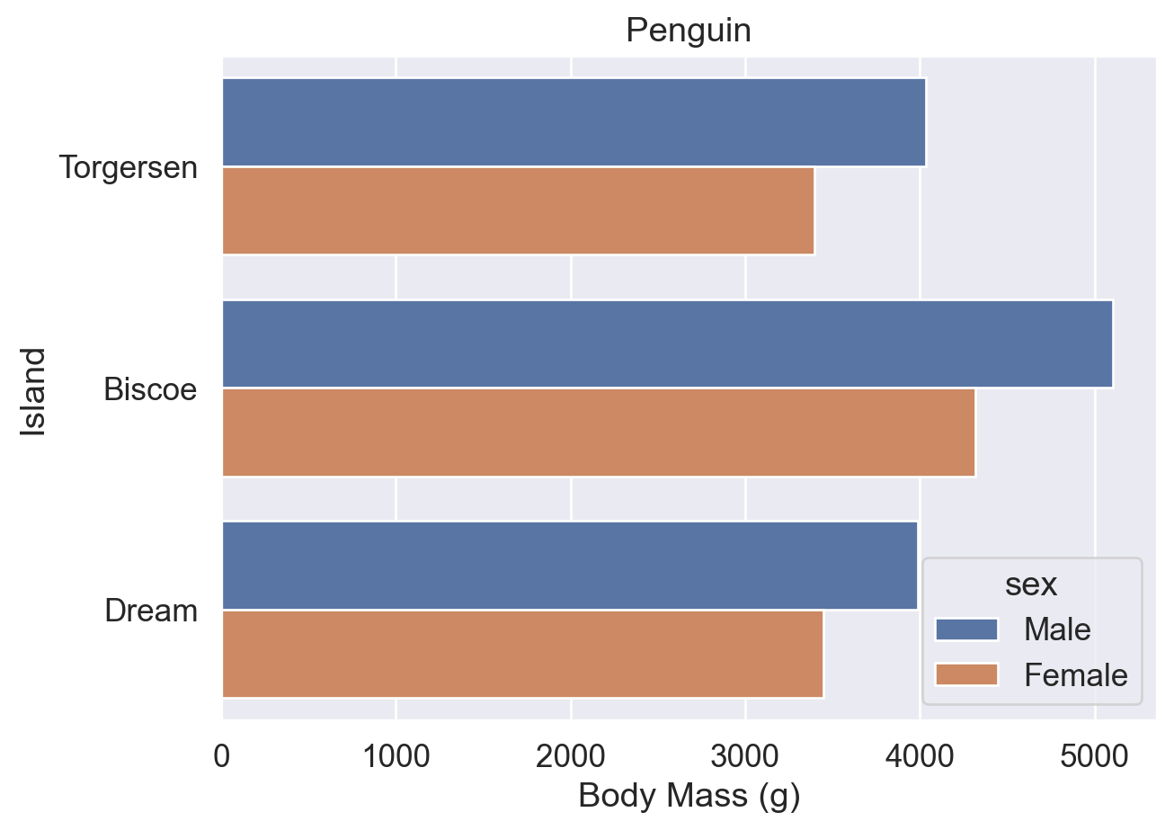
After assigning a Seaborn chart to the variable ax, you can call Matplotlib methods on it for further customization, similar to assigning a DataFrame to df and then calling its methods.
Note the difference between these two:
sns.set() / sns.set_theme(): Seaborn global theme-setting functions. They are equivalent, but sns.set_theme() is preferred.ax.set(): a Matplotlib method for a specific chart object, used to set titles, axis labels, and related elements.References:
sns.set() documentation
sns.set_theme() documentation
ax.set() documentation
Whether you use errorbar=None or errorbar=('ci', 0), the legend may cover the plot, so you may need to adjust its position manually with sns.move_legend().
# errorbar=None: the legend is automatically placed on the right
ax = sns.barplot(data=df, y='island', x='body_mass_g', errorbar=None, hue='sex')
ax.set(title='Penguin', xlabel='Body Mass (g)', ylabel='Island')
plt.show()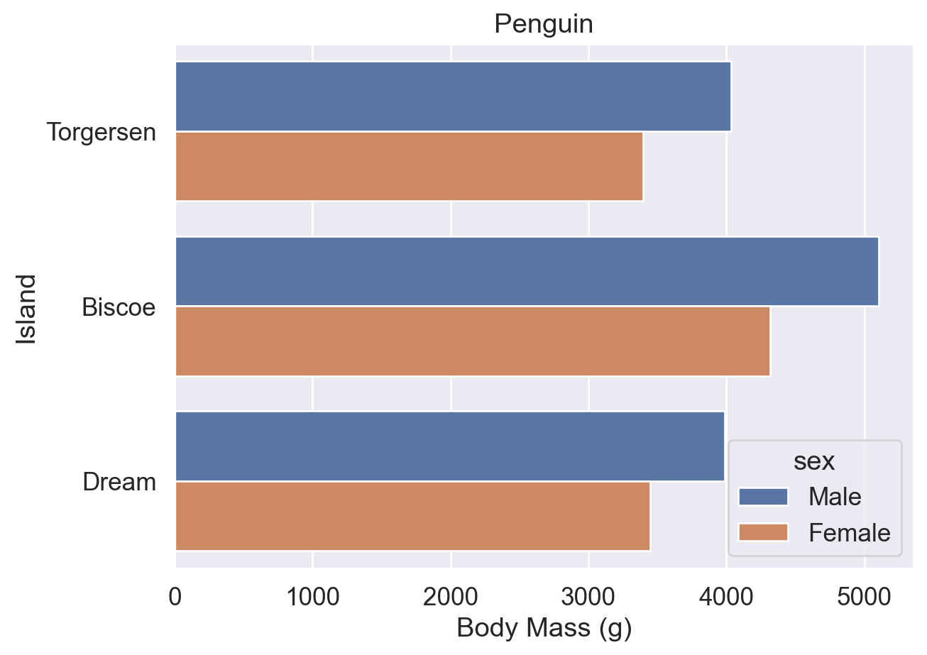
# errorbar=('ci', 0): the legend is automatically moved away from the error-bar area
ax = sns.barplot(
    data=df, y='island', x='body_mass_g',
    errorbar=('ci', 0), hue='sex',
)
ax.set(title='Penguin', xlabel='Body Mass (g)', ylabel='Island')
plt.show()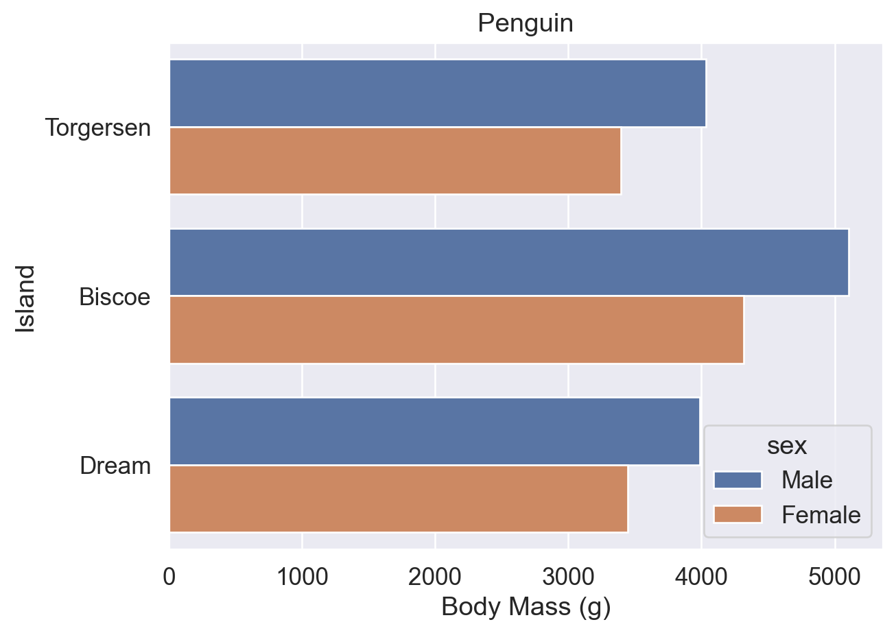
ax = sns.barplot(data=df, y='island', x='body_mass_g', errorbar=None, hue='sex')
ax.set(title='Penguin', xlabel='Body Mass (g)', ylabel='Island')

# Combine bbox_to_anchor with loc: move the legend's loc reference point to (0.5, -0.2)
sns.move_legend(ax, bbox_to_anchor=(0.5, -0.2), loc='upper center', ncols=2)
plt.show()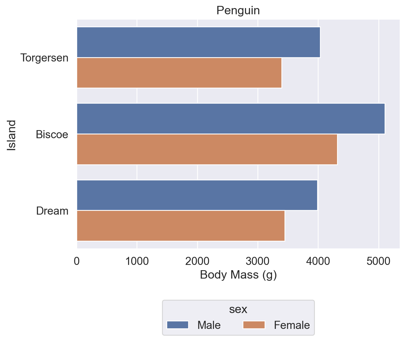
ax = sns.barplot(data=df, y='island', x='body_mass_g', errorbar=None, hue='sex')
ax.set(title='Penguin', xlabel='Body Mass (g)', ylabel='Island')
sns.move_legend(ax, loc='lower right')  # Set loc only: move the legend to the lower right of the plot
plt.show()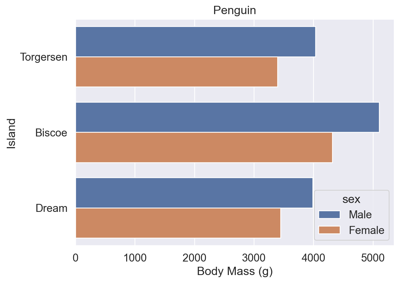
ax = sns.barplot(data=df, y='island', x='body_mass_g', errorbar=None, hue='sex')
ax.set(title='Penguin', xlabel='Body Mass (g)', ylabel='Island')

# Place the upper-left corner of the legend at (1, 1) relative to the axes
sns.move_legend(ax, loc='upper left', bbox_to_anchor=(1, 1))
plt.show()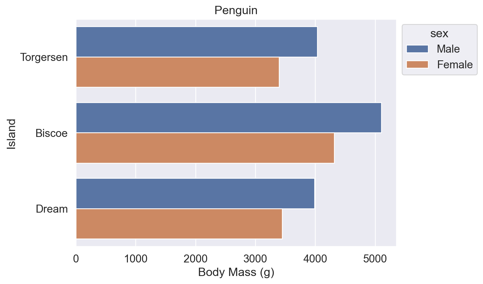
References:
sns.move_legend() documentation (obj and loc parameters)
matplotlib.axes.Axes.legend() documentation (loc, ncols, and bbox_to_anchor parameters)
Use the palette parameter to change chart colors. It can take the following kinds of values:
'deep'): 'deep', 'muted', 'bright', 'pastel', 'dark', 'colorblind''viridis', 'plasma', 'coolwarm', 'Blues', 'Reds''hls', 'husl''ch:<args>', for example 'ch:s=0.5,r=-0.5' (colorblind-friendly and suitable for grayscale printing)'light:<color>', 'dark:<color>''blend:<color1>,<color2>'['#FF5733', '#33FF57'], RGB tuples, or Matplotlib color names# Default palette
ax = sns.barplot(data=df, y='island', x='body_mass_g', errorbar=None, hue='sex')
ax.set(title='Penguin', xlabel='Body Mass (g)', ylabel='Island')
sns.move_legend(ax, bbox_to_anchor=(1, 1), loc='upper left')
plt.show()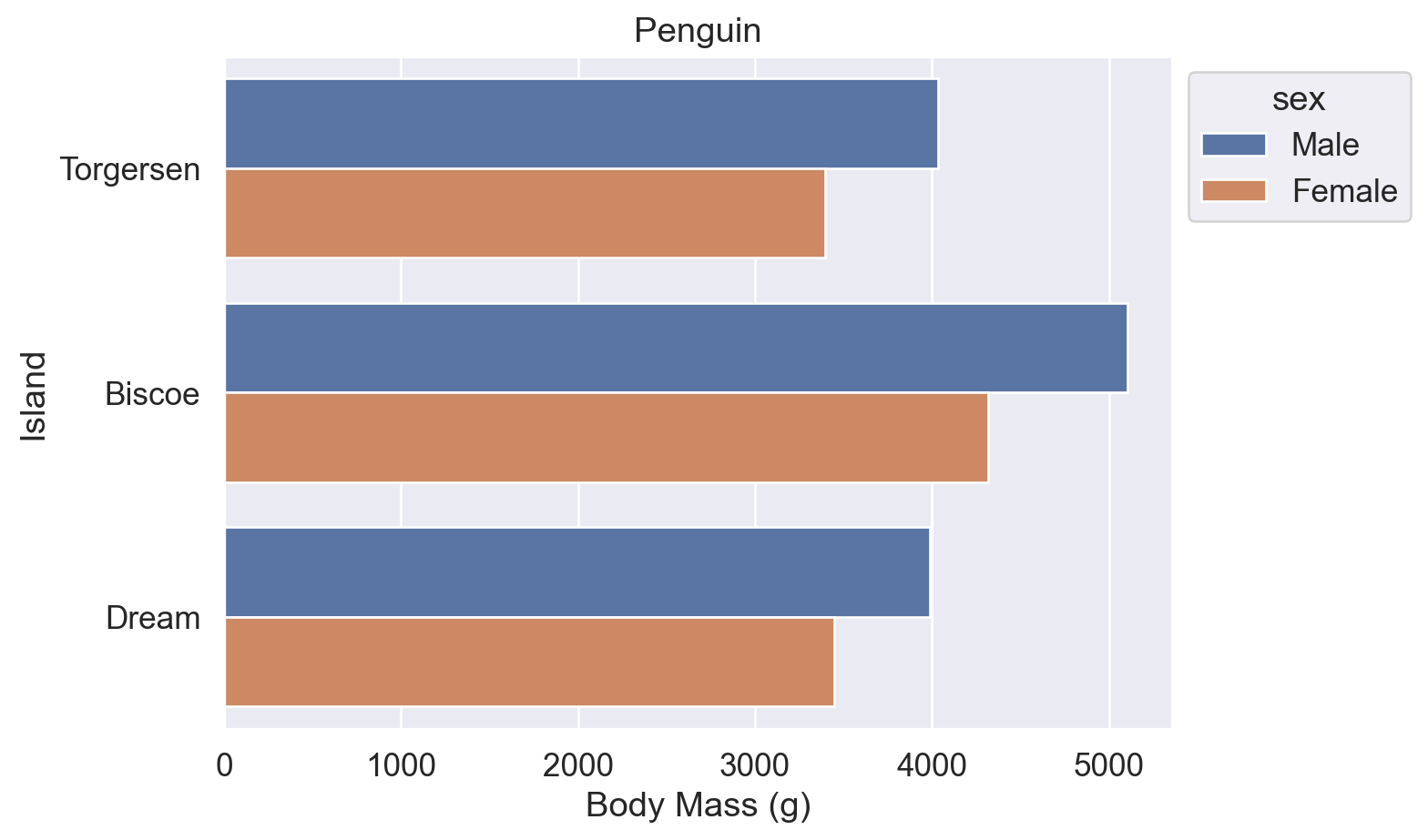
# palette='flare': use a predefined Seaborn palette
ax = sns.barplot(data=df, y='island', x='body_mass_g', errorbar=None, hue='sex', palette='flare')
ax.set(title='Penguin', xlabel='Body Mass (g)', ylabel='Island')
sns.move_legend(ax, bbox_to_anchor=(1, 1), loc='upper left')
plt.show()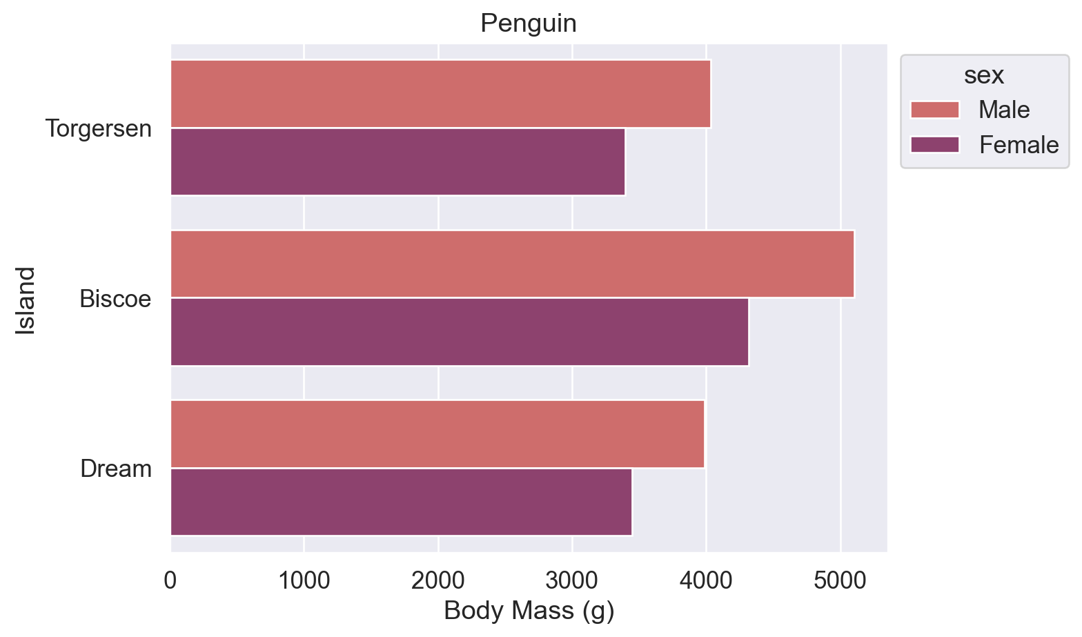
# Pass a list of Matplotlib color names to palette
ax = sns.barplot(data=df, y='island', x='body_mass_g', errorbar=None, hue='sex', palette=['blue', 'orange'])
ax.set(title='Penguin', xlabel='Body Mass (g)', ylabel='Island')
sns.move_legend(ax, bbox_to_anchor=(1, 1), loc='upper left')
plt.show()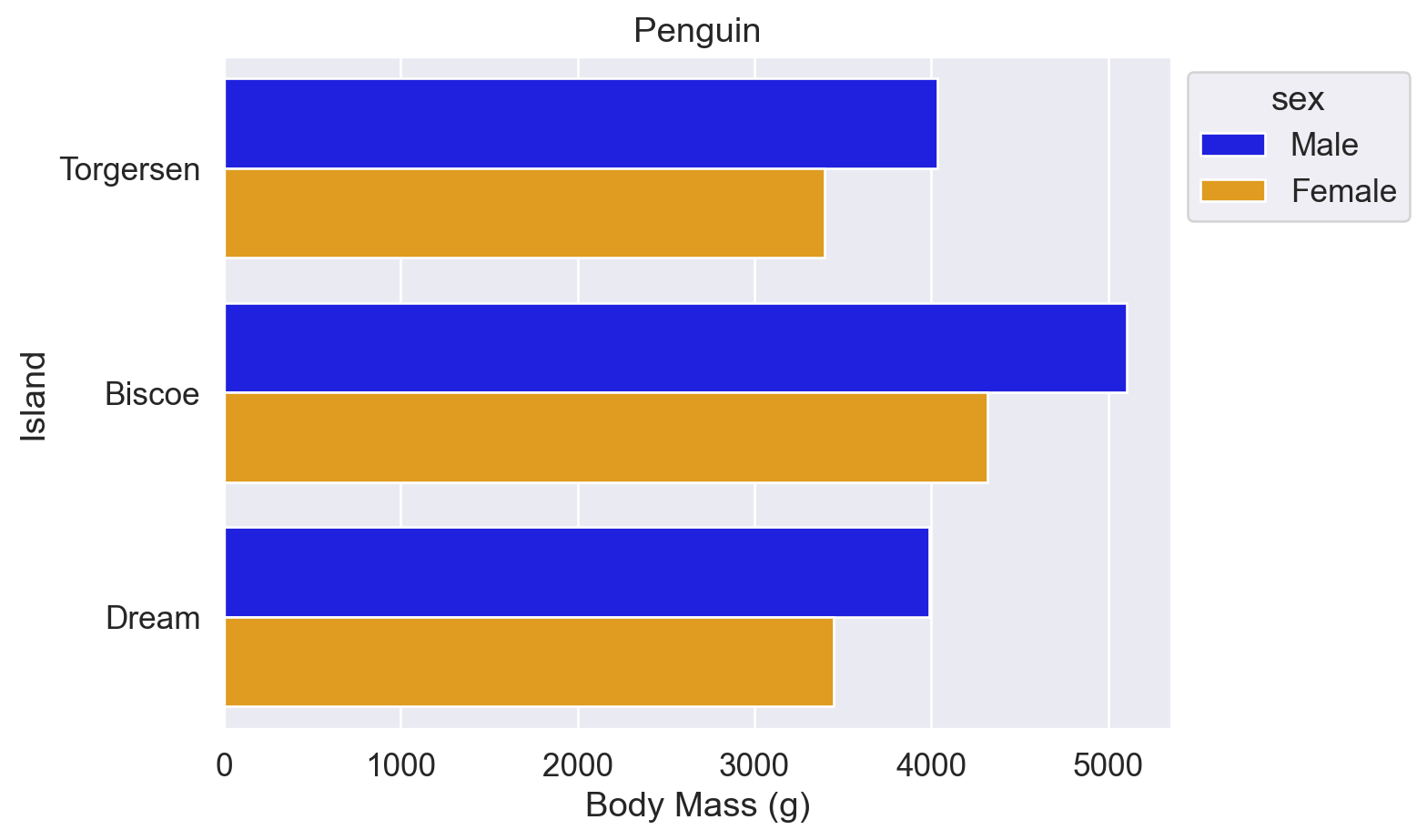
# Pass a list of hexadecimal color codes to palette
ax = sns.barplot(
    data=df, y='island', x='body_mass_g',
    errorbar=None, hue='sex', palette=['#a1c9f4', '#8de5a1'],
)
ax.set(title='Penguin', xlabel='Body Mass (g)', ylabel='Island')
sns.move_legend(ax, bbox_to_anchor=(1, 1), loc='upper left')
plt.show()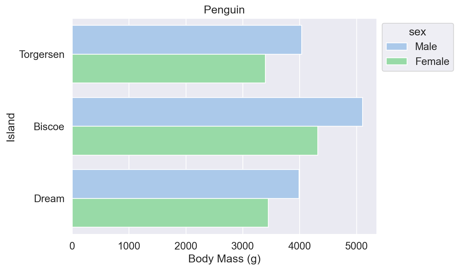
References:
Seaborn sns.set_theme() documentation (palette parameter)
Seaborn sns.color_palette() documentation (list of predefined palette names)
Matplotlib named colors
Matplotlib colormaps
w3schools color picker
The following two approaches are equivalent and can be used later to sort bar plots by totals.
Method 1: df.groupby().size()
# Group by island and count the number of rows in each group
df.groupby('island').size()
island
Biscoe 168
Dream 124
Torgersen 52
dtype: int64Method 2: df.value_counts()
# Count the occurrences of each value in the island column
df.value_counts('island')
island
Biscoe 168
Dream 124
Torgersen 52
Name: count, dtype: int64The y-axis of a bar plot must start at 0 to ensure that the visual proportions match the data proportions, following Wilke’s Principle of Proportional Ink (Wilke 2019, chap. 17). Point plots do not have this restriction: the y-axis can start from the data range, and the data-ink ratio is higher because there is less visual clutter.
When the x-axis is nominal data, such as island names, the points do not need to be connected with lines.
# linestyle='none': do not connect points when the x-axis is categorical.
# The vertical segments around points are error bars.
sns.pointplot(data=df, x='island', y='body_mass_g', hue='sex', linestyle='none')
plt.show()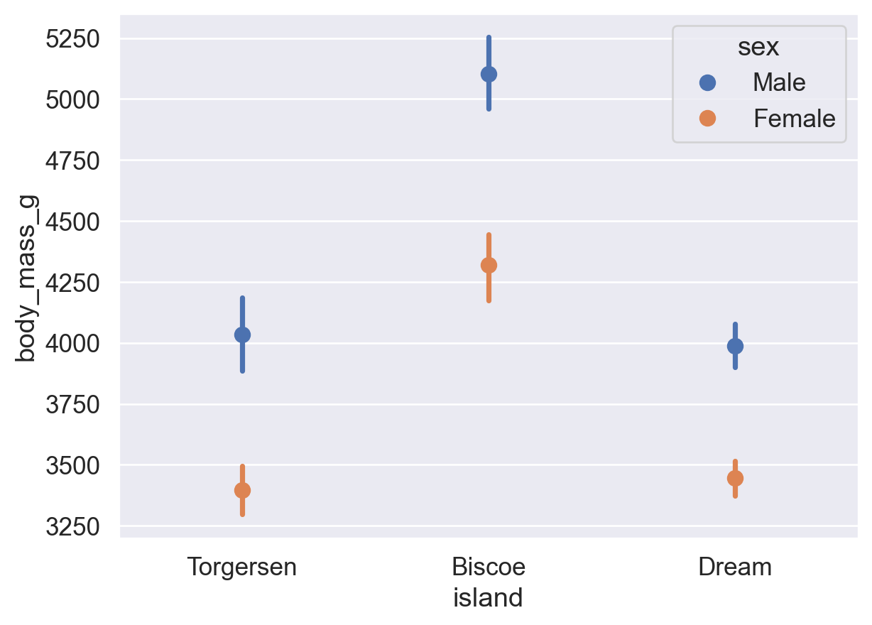
Reference: sns.pointplot() documentation
The x-axis of a bar plot represents discrete categories (nominal or ordinal data). The x-axis of a histogram represents continuous numerical intervals (ratio data).
sns.histplot(data=df, x='flipper_length_mm')
plt.show()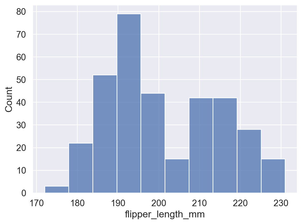
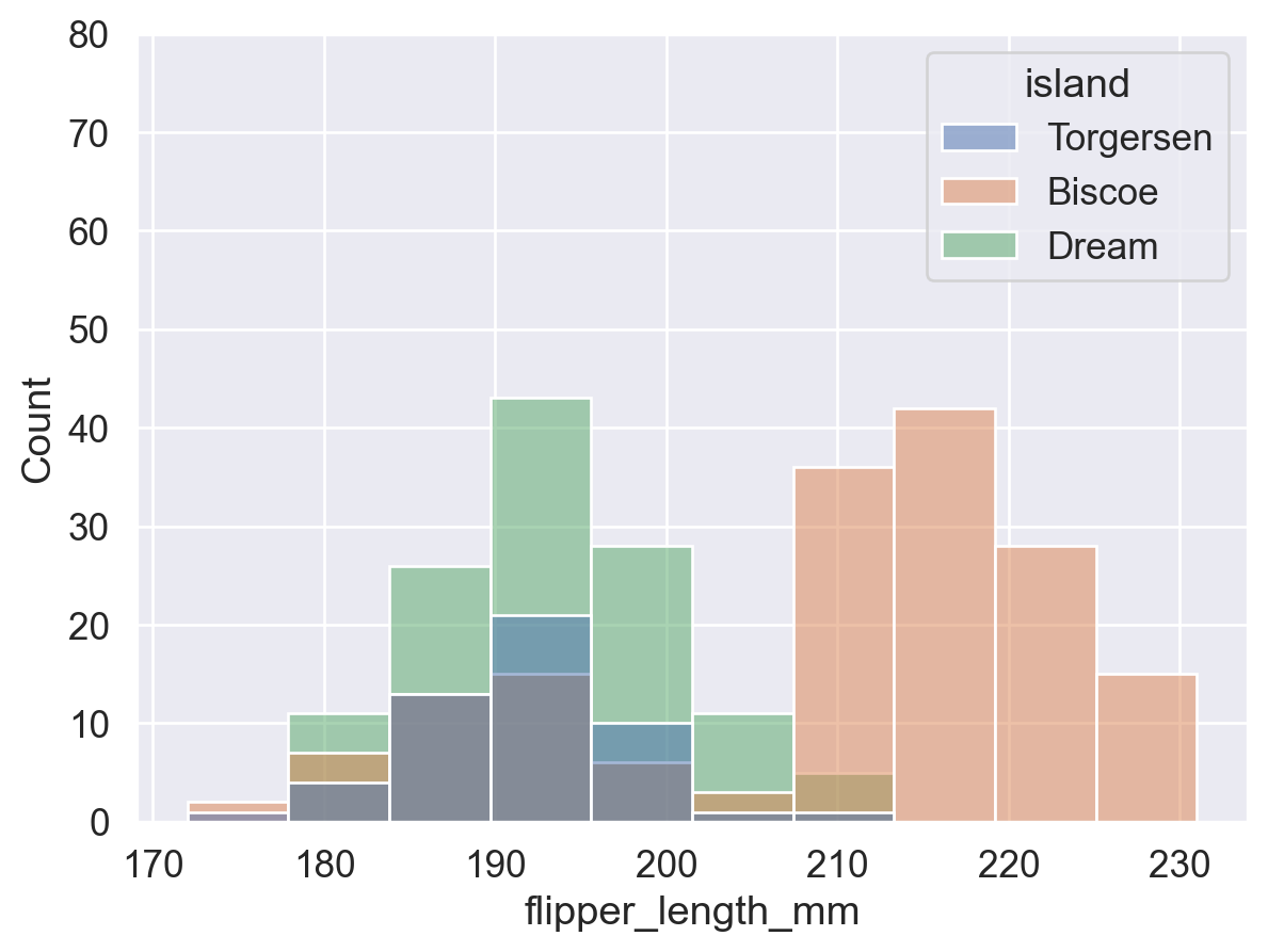
# Group with hue: plot penguins from each island separately and overlay the distributions
sns.histplot(data=df, x='flipper_length_mm', hue='island')
plt.show()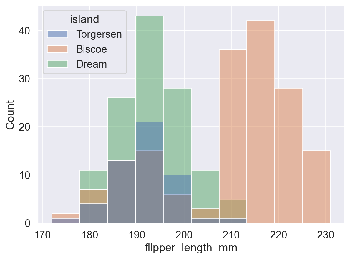
# Use a consistent y-axis range to compare the plot with and without hue grouping
sns.histplot(data=df, x='flipper_length_mm')
plt.show()

sns.histplot(data=df, x='flipper_length_mm', hue='island')
plt.ylim(0, 80)
plt.show()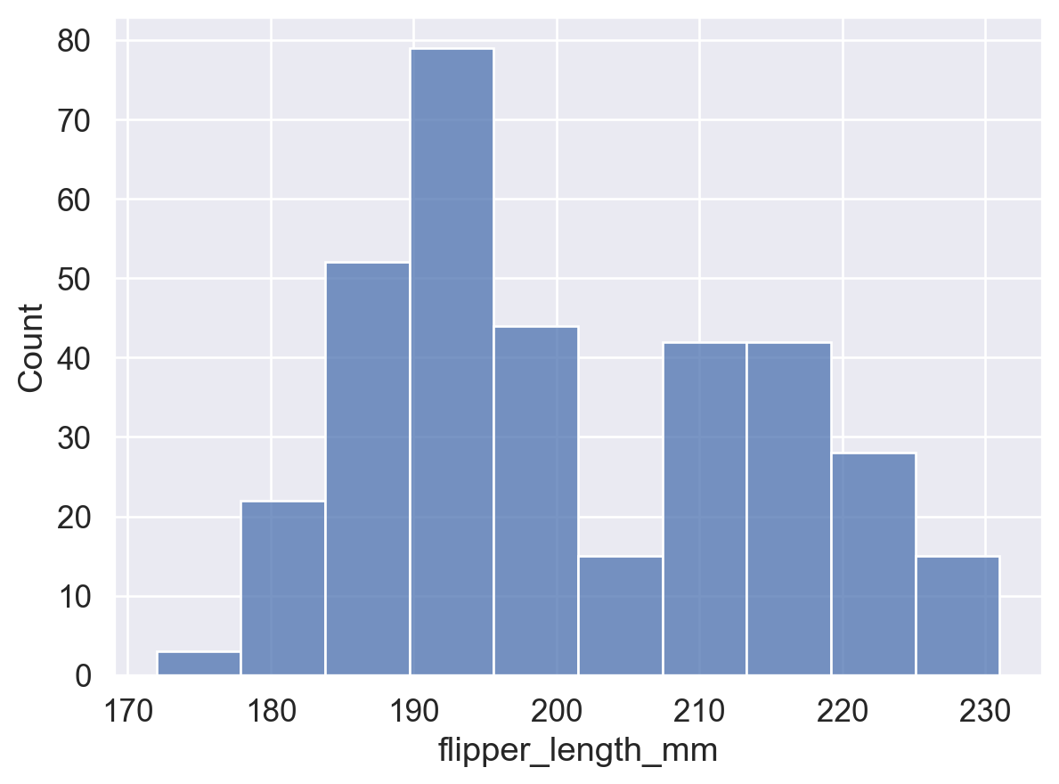
sns.histplot(
    data=df, x='flipper_length_mm',
    hue='island',
    stat='density',     # The total area of all bins is 1 (probability density)
    common_norm=False   # Normalize each group separately. If True, all groups share one total area of 1.
)
plt.show()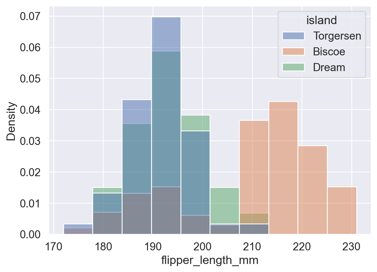
stat ParameterThis parameter controls the statistic shown by the histogram. Available values include:
'count': bin height = number of data points in the bin.'frequency': bin height = count / bin width, or frequency per unit width. This is useful when bin widths are unequal.'probability' / 'proportion': bin height = count / total count, so all bin heights sum to 1.'percent': bin height = (count / total count) * 100, so all bin heights sum to 100.'density': bin height = frequency / bin width, so the total area of all bins is 1. As bin width approaches 0, this becomes a smooth density curve.# stat='count': bar height = number of data points in each bin
ax = sns.histplot(data=df, x='flipper_length_mm', stat='count')
# Iterate over each bar (patch), get its height, and show a value label above it
for p in ax.patches:
# Get the bar height, which is the frequency in the interval
height = p.get_height()
# Add text
ax.text(
p.get_x() + p.get_width() / 2, # x coordinate: center of the bar
height, # y coordinate: bar height
int(height), # text: integer frequency
ha='center', va='bottom', # horizontal/vertical alignment
)
plt.show()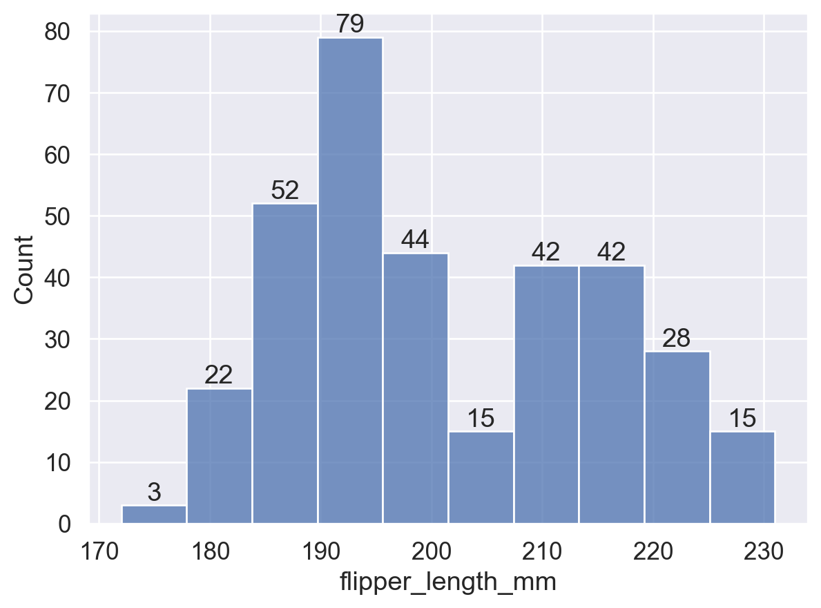
# stat='frequency': bar height = count / bin width
ax = sns.histplot(data=df, x='flipper_length_mm', stat='frequency')
for p in ax.patches:
    height = p.get_height()
    ax.text(
        p.get_x() + p.get_width() / 2,
        height, int(height),
        ha='center', va='bottom',
    )
plt.show()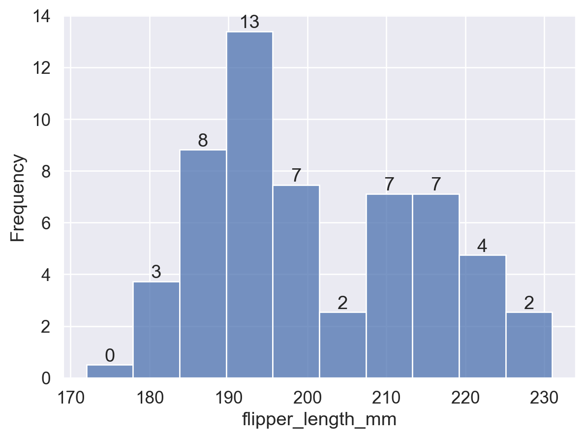
# stat='probability': bar height = count / total count, and all bar heights sum to 1
ax = sns.histplot(data=df, x='flipper_length_mm', stat='probability')
for p in ax.patches:
    height = p.get_height()
    ax.text(
        p.get_x() + p.get_width() / 2,
        height, f'{height:.2f}', # Keep two decimal places
        ha='center', va='bottom',
    )
plt.show()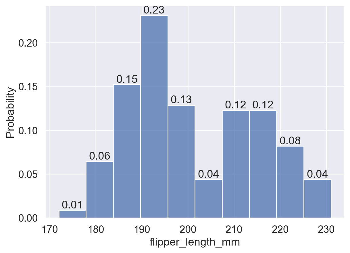
# stat='percent': bar height = (count / total count) * 100, and all bar heights sum to 100
ax = sns.histplot(data=df, x='flipper_length_mm', stat='percent')
for p in ax.patches:
    height = p.get_height()
    ax.text(
        p.get_x() + p.get_width() / 2,
        height, int(height),
        ha='center', va='bottom',
    )
plt.show()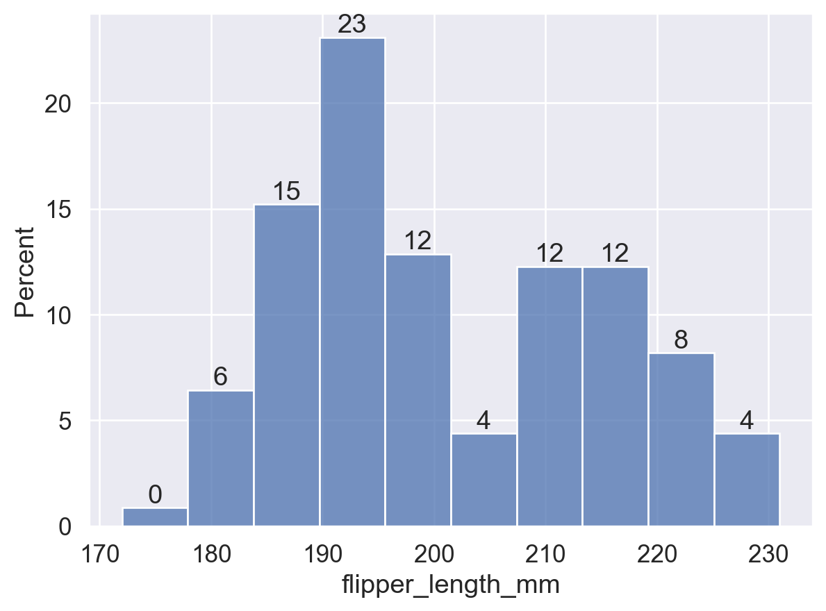
# stat='density': bar height = frequency / bin width, and the total bin area is 1
ax = sns.histplot(data=df, x='flipper_length_mm', stat='density')
for p in ax.patches:
    height = p.get_height()
    ax.text(
        p.get_x() + p.get_width() / 2,
        height, f'{height:.3f}',
        ha='center', va='bottom',
    )
plt.show()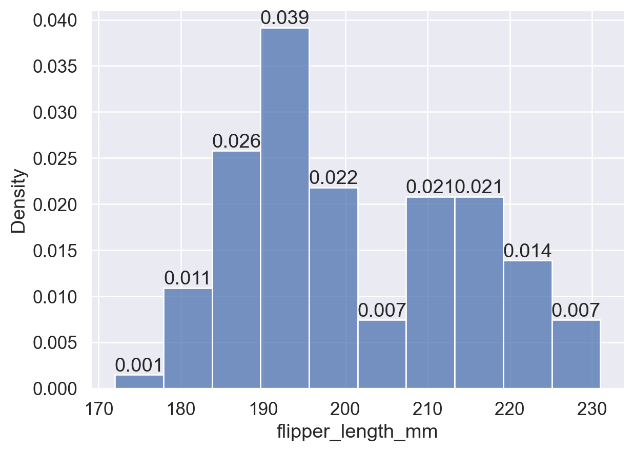
common_norm ParameterThis boolean parameter only applies when stat is 'probability', 'proportion', 'percent', or 'density'. Its default value is True:
common_norm=True: normalize using the entire dataset, so bin heights can be compared across groups.common_norm=False: normalize each subgroup independently, so bin heights are only meaningful within each group.sns.histplot(
data=df, x='flipper_length_mm', hue='island',
stat='density', common_norm=True, # Overall normalization: the total bin area across all groups is 1
)
plt.show()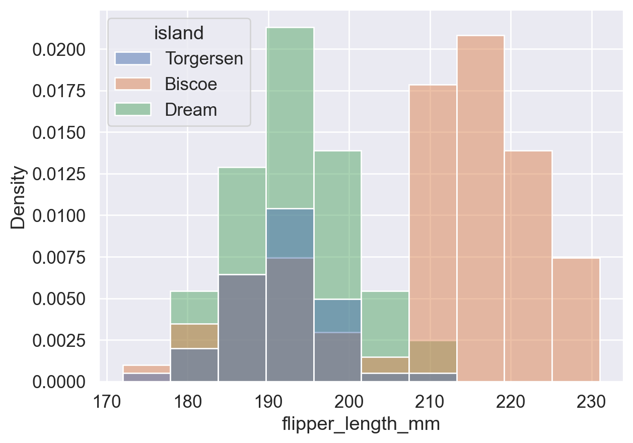
sns.histplot(
    data=df, x='flipper_length_mm', hue='island',
    stat='density', common_norm=False, # Separate normalization: each group's bin area sums to 1
)
plt.show()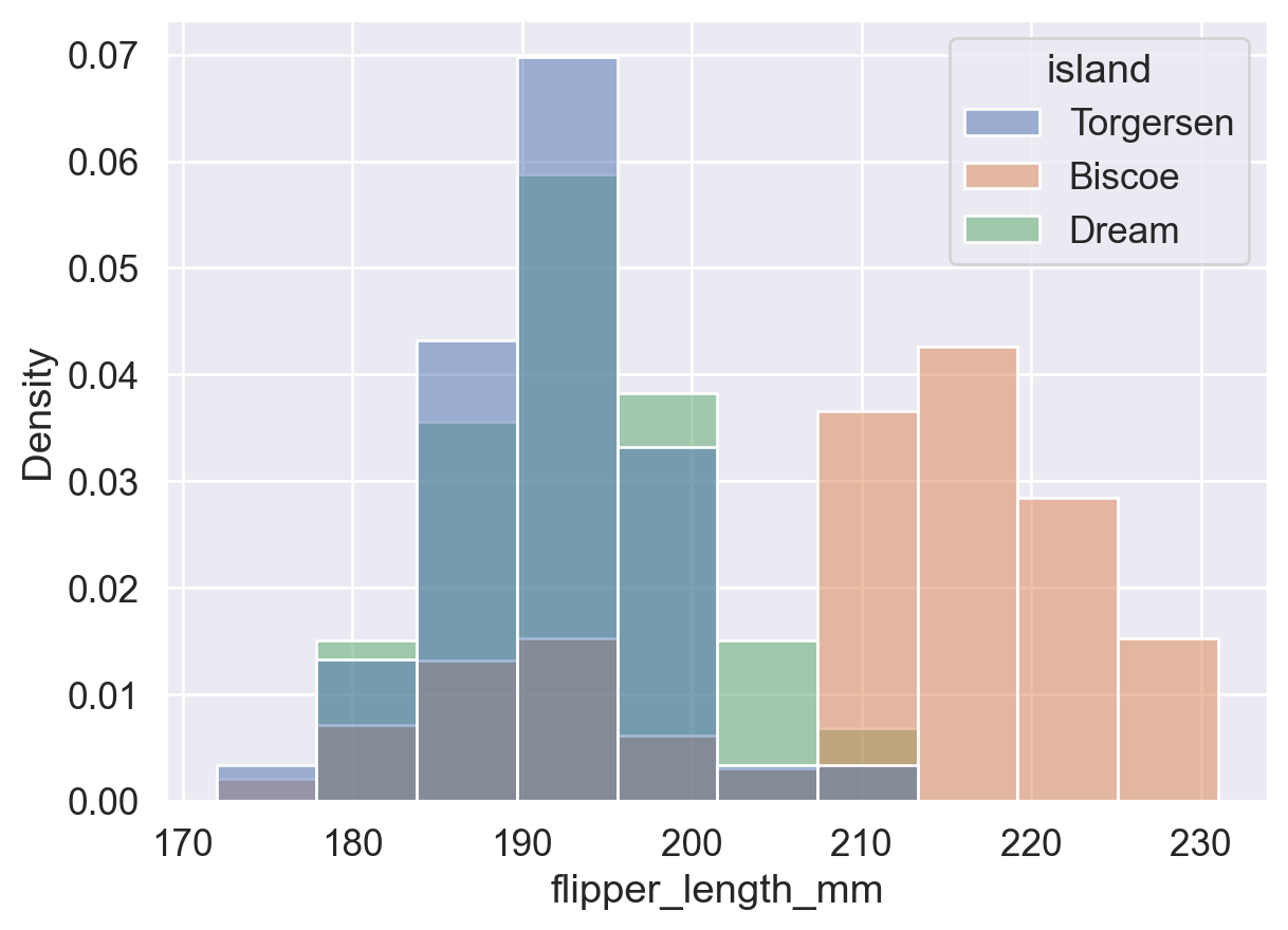
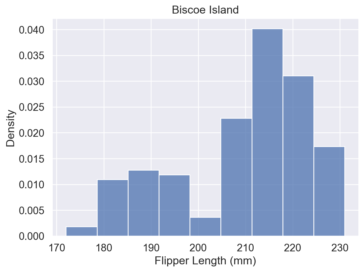
When overlapping groups are difficult to read, use data=df[df['column']==value] to filter the data and plot each group separately:
# Plot by island to avoid overlapping groups and inspect each island's distribution separately
ax = sns.histplot(
    data=df[df['island'] == 'Torgersen'],
    x='flipper_length_mm', stat='density'
)
ax.set(title='Torgersen Island', xlabel='Flipper Length (mm)')
plt.show()

ax = sns.histplot(
    data=df[df['island'] == 'Biscoe'],
    x='flipper_length_mm', stat='density'
)
ax.set(title='Biscoe Island', xlabel='Flipper Length (mm)')
plt.show()

ax = sns.histplot(
    data=df[df['island'] == 'Dream'],
    x='flipper_length_mm', stat='density'
)
ax.set(title='Dream Island', xlabel='Flipper Length (mm)')
plt.show()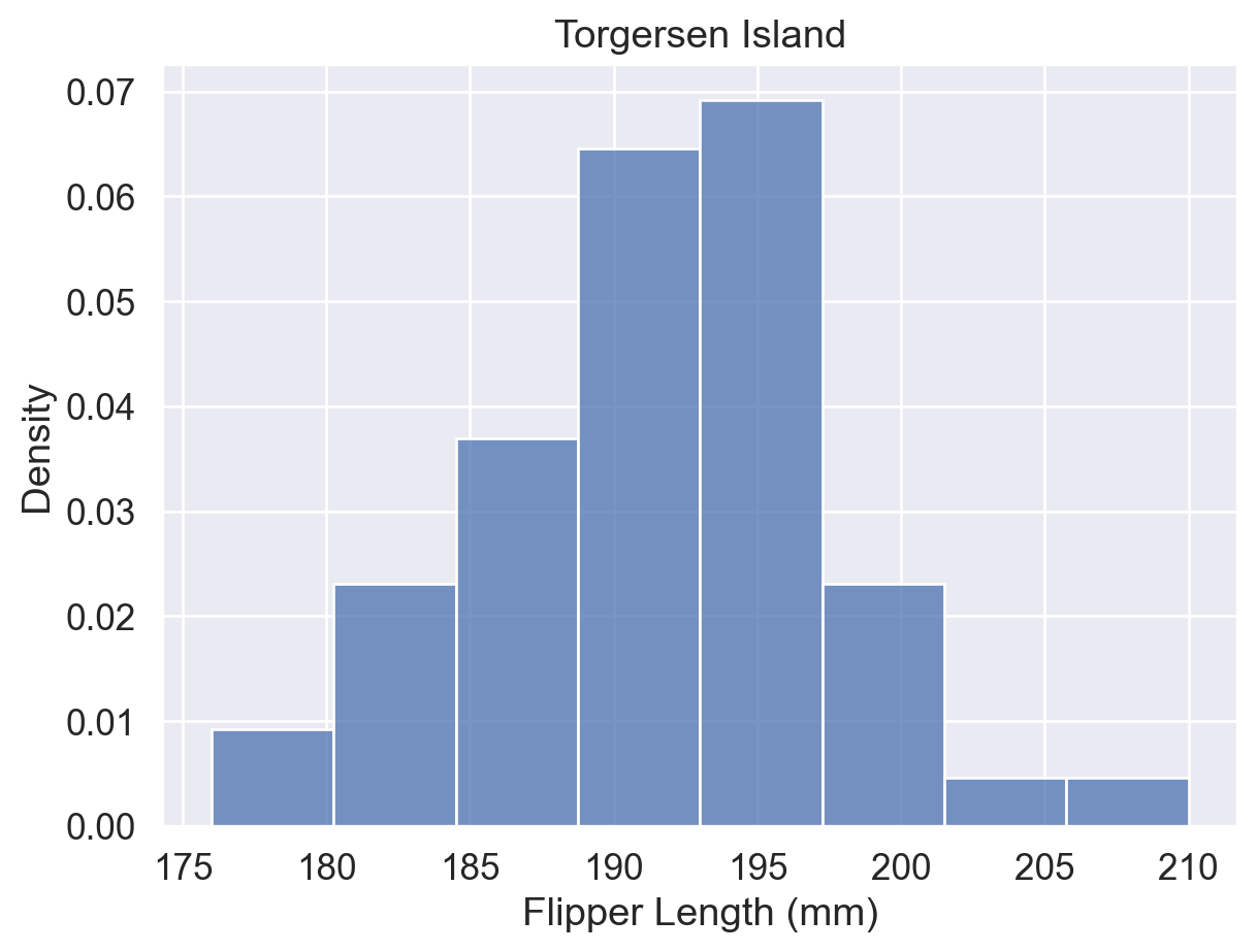
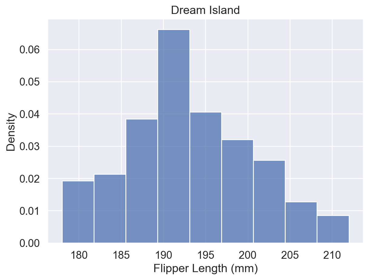
Reference: sns.histplot() documentation (hue, stat, and common_norm parameters)
A box plot summarizes a distribution with five key values: min, Q1, Q2 (median), Q3, and max. It also marks outliers beyond the whisker range.
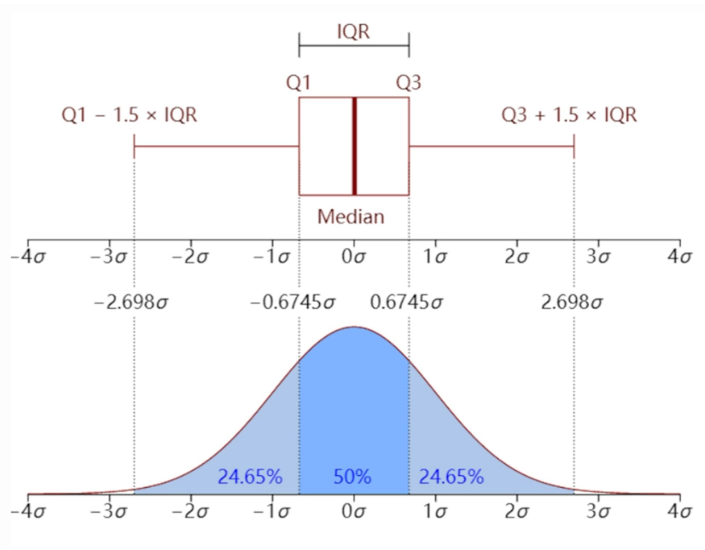
Box Plot vs. Histogram
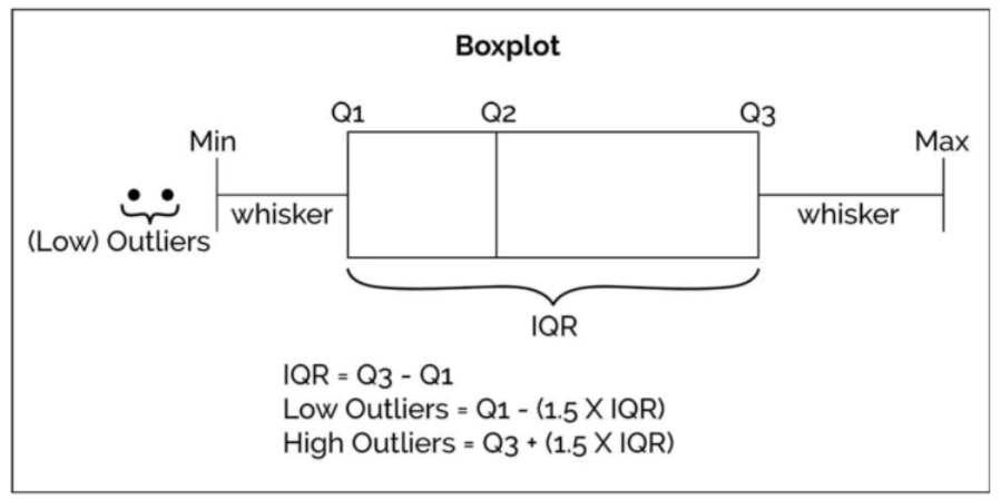
Box plots are useful for quickly identifying a distribution summary and outliers. Histograms are better for seeing the frequency distribution within specific intervals.
sns.boxplot(data=df, x='flipper_length_mm', y='island', hue='sex')
plt.show()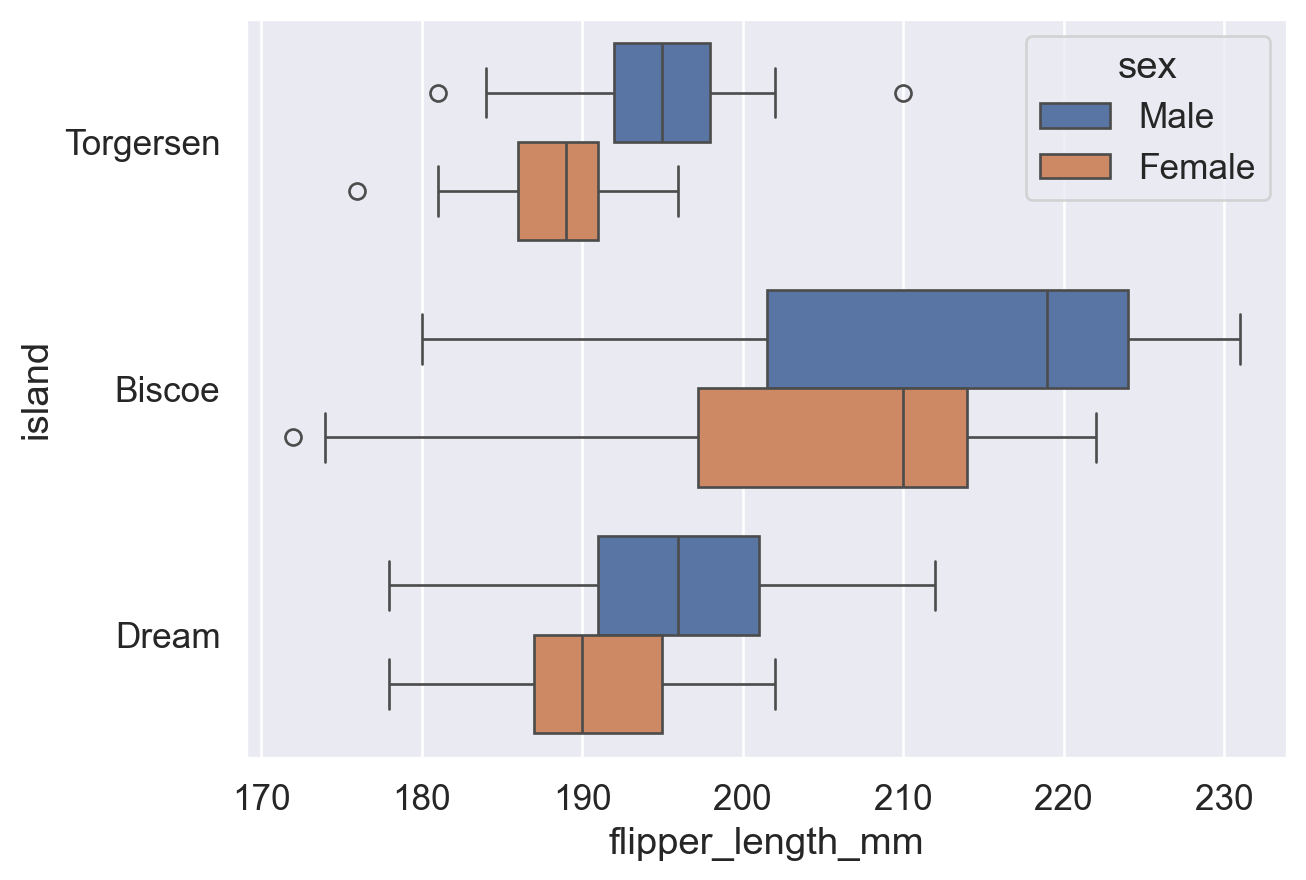
sns.boxplot(
    data=df, x='flipper_length_mm', y='island', hue='sex',
    fliersize=8,  # fliersize: size of outlier points (default: 5)
)
plt.show()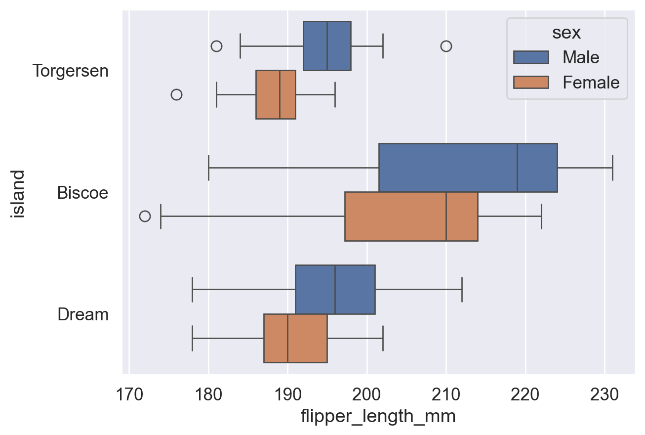
sns.boxplot(
    data=df, x='flipper_length_mm', y='island', hue='sex', fliersize=8,
    whis=2,  # whisker: extend to Q1/Q3 +/- 2*IQR (default: 1.5); larger values reduce outlier points
)
plt.show()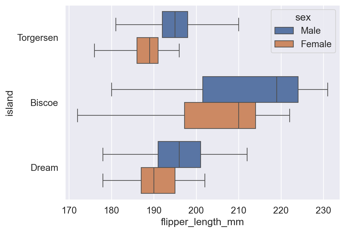
Reference: sns.boxplot() documentation (fliersize and whis parameters)
A violin plot combines features of a box plot, such as medians and quantiles, with a density curve that shows the smoothed distribution. When the dataset is small, the smoothed curve may be misleading, so a histogram or box plot may be preferable.
sns.violinplot(data=df, y='island', x='flipper_length_mm', hue='sex')
plt.show()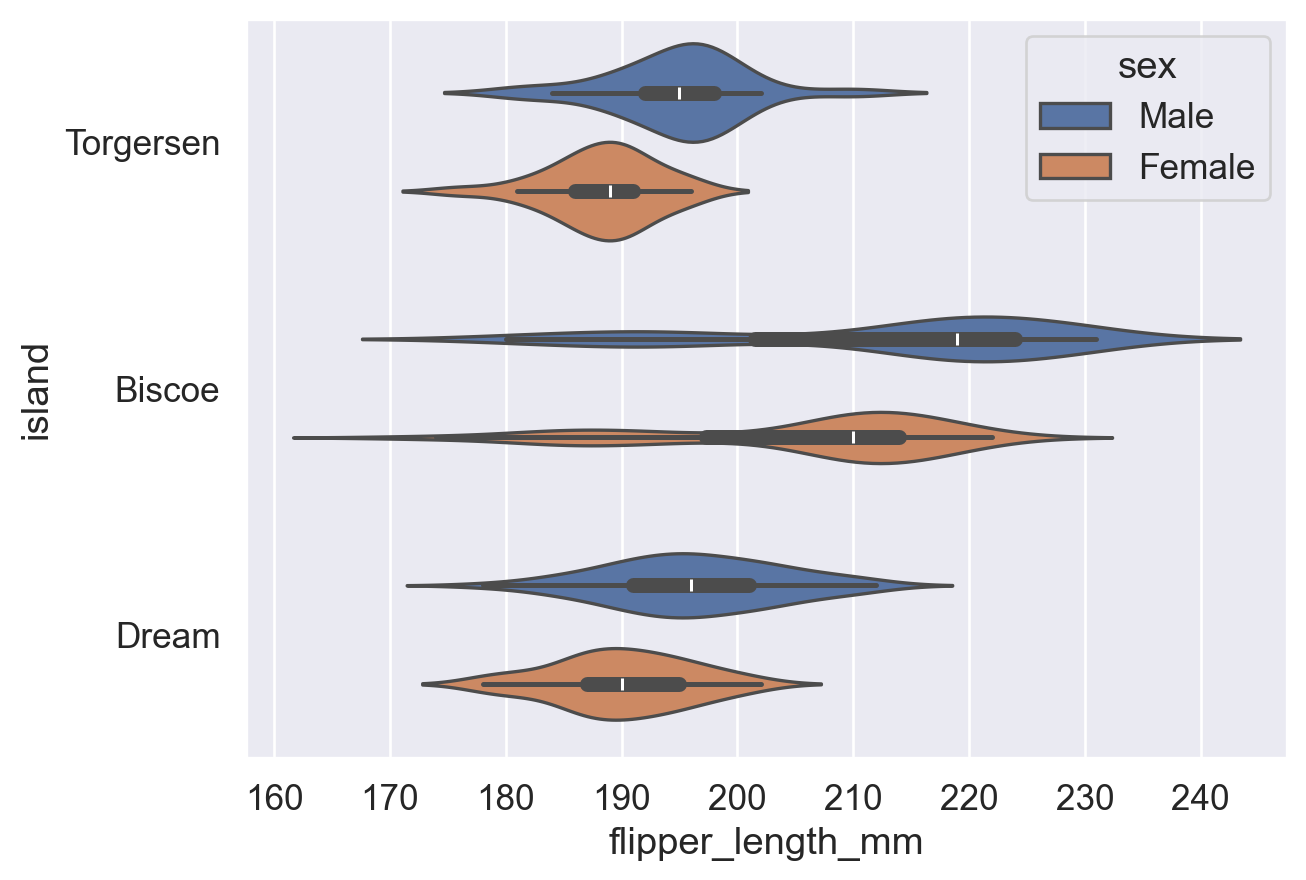
# split=True: combine the two hue groups in the same category into one violin for easier distribution comparison
sns.violinplot(
    data=df, y='island', x='flipper_length_mm', hue='sex',
    split=True, # Combine two hue groups into one violin for easier comparison
)
plt.show()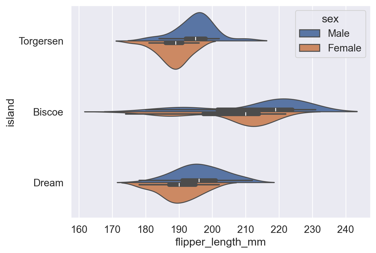
Reference: sns.violinplot() documentation (split parameter)
Strip plots draw every data point, with each dot representing one observation. Points are randomly jittered along the categorical axis to reduce overlap. Swarm plots automatically arrange overlapping data points and are easier to read.
Note that both plots show a univariate distribution, meaning how densely one variable appears across its range. This is different from a scatter plot, which shows the relationship between two variables.
| Comparison | Strip Plot | Swarm Plot |
|---|---|---|
| Basic idea | Randomly jitter data points along the categorical axis to avoid overlap | Precisely arrange points with an algorithm to avoid overlap and show the distribution |
| Point placement | Random jitter; overlap may still occur | Non-random; automatically adjusted by density to avoid overlap |
| Readability | Clear for small datasets; can overlap heavily with large datasets | Clearer for showing distribution shape in small to medium datasets |
| Computational cost | Lower and faster to draw | Higher and slower for large datasets |
| Suitable uses | Quick visualization, small datasets, situations where exact distribution shape is less important | Showing distribution details for medium-sized datasets |
| Distribution detail | Moderate; true density can be hard to see | Stronger; data density is easier to read visually |
| Parameter control | Jitter can be controlled with jitter |
No jitter needed; the algorithm adjusts placement automatically |
| Example function | sns.stripplot() |
sns.swarmplot() |
sns.stripplot(data=df, x='flipper_length_mm', y='island', hue='sex')
plt.show()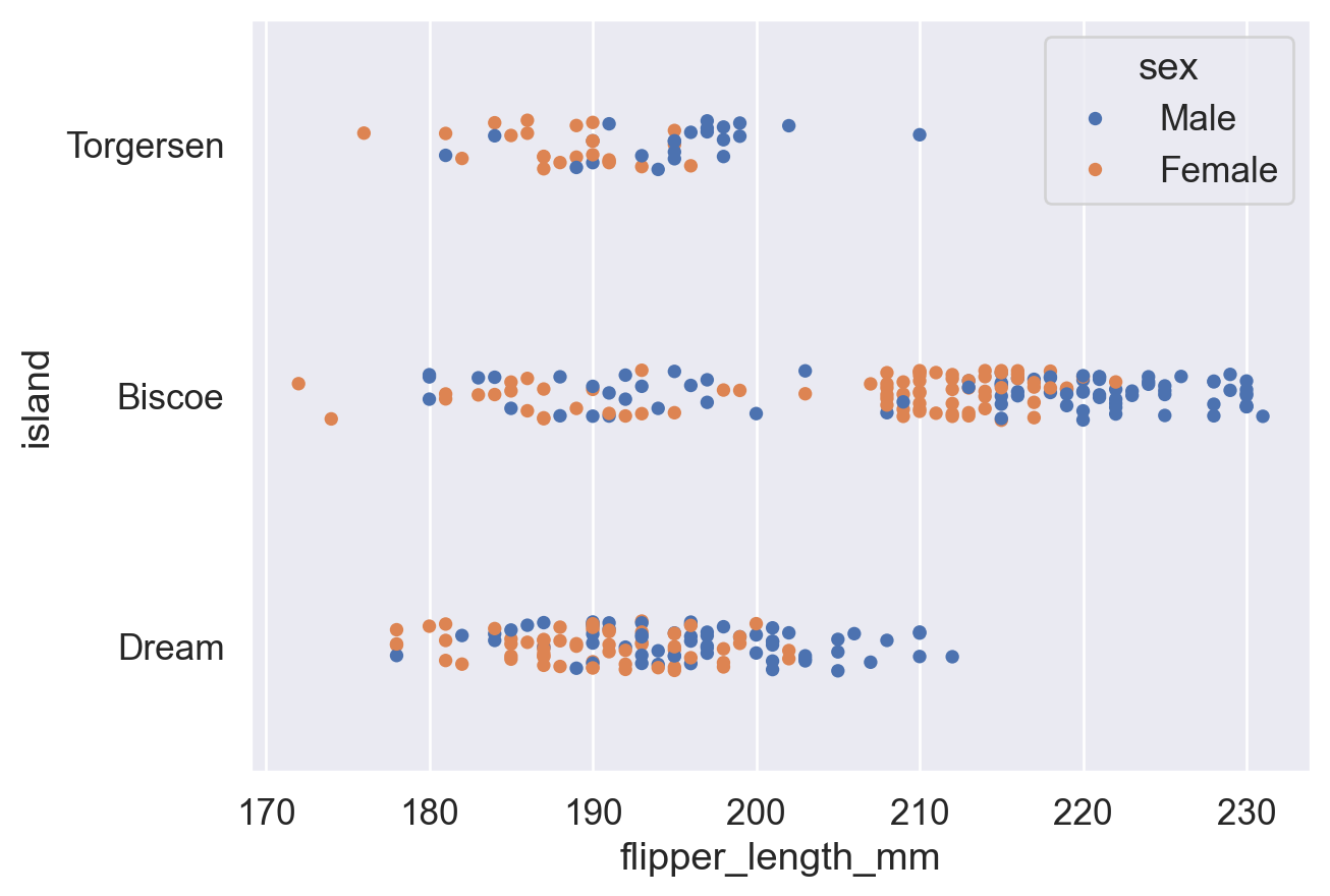
sns.swarmplot(data=df, x='flipper_length_mm', y='island', hue='sex')
plt.show()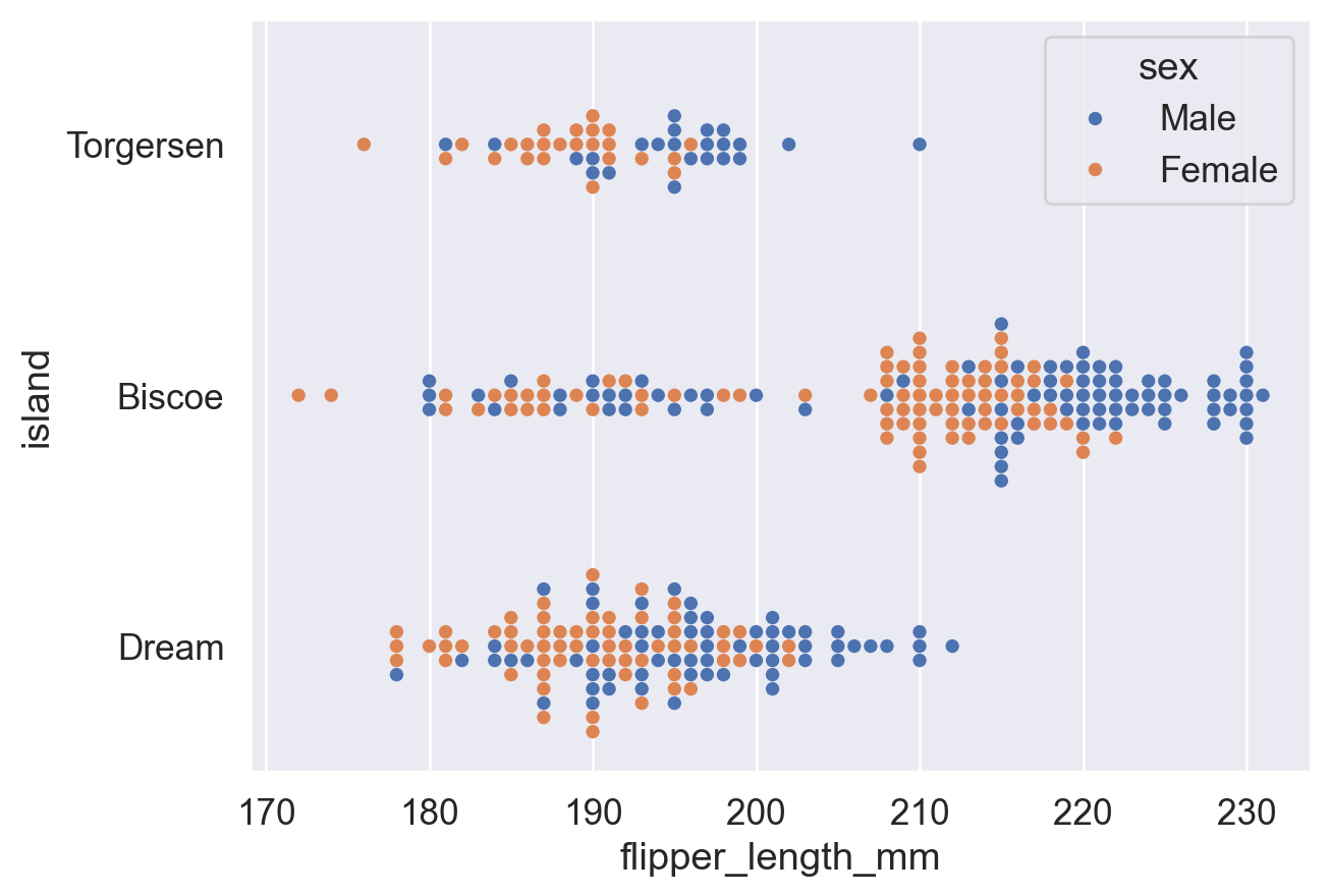
References:
sns.stripplot() documentation
sns.swarmplot() documentation
General links:
Python 3 documentation (for built-in functions and related usage)
Pandas documentation (DataFrame)
Matplotlib documentation (plt)
Seaborn documentation (barplot)
sns.barplot()documentation (drawing bar plots with Seaborn)
sns.countplot()documentation (drawing count plots with Seaborn)Changing chart themes:
plt.xticks()documentation (thekwargssection explains how to rotate tick labels)
sns.set()documentation (equivalent tosns.set_theme())
sns.set_theme()documentation (set the global Seaborn plotting theme)
ax.set()documentation (set titles, axis labels, and related elements for a specific Matplotlib axes object)Changing legends:
sns.move_legend()documentation (Seaborn function for moving legends; see theobjandlocparameters)
matplotlib.axes.Axes.legend()documentation (Matplotlib legend function; its options also apply tosns.move_legend(); seeloc,ncols, andbbox_to_anchor)Changing chart colors:
Seabornsns.color_palette()documentation (predefined palette names for thepaletteparameter)
Matplotlib named colors
Matplotlib colormaps
Matplotlib colormap guide
w3schools color picker (view hexadecimal codes for colors)Other charts:
sns.pointplot()documentation (drawing point plots)
sns.histplot()documentation (drawing histograms; seehue,stat, andcommon_norm)
sns.boxplot()documentation (drawing box plots; seefliersizeandwhis)
sns.violinplot()documentation (drawing violin plots)
sns.stripplot()documentation (drawing distribution scatter plots)
sns.swarmplot()documentation (drawing clustered distribution scatter plots)Textbook: Fundamentals of Data Visualization (Wilke, 2019):
6.1 Bar Plot (rotated tick labels are harder to read; a horizontal layout is preferable)
17. The Principle of Proportional Ink (the proportions of graphical marks should match the true proportions in the data; for example, bars in a bar plot should start from 0)