Evolution of Online AI Discourse

NLP

Text Analysis

Social Media

A Longitudinal Analysis of Public Sentiment and Thematic Trends in AI-Related Tweets

Author

Pinn Xu

Published

May 1, 2026

29 min read · 5676 EN words · 0 中文字

Environment & Versions

R==4.5.2
MASS==7.3.65
tidyverse==2.0.0
tidytext==0.4.3
textdata==0.4.5
topicmodels==0.2.17
scales==1.4.0
broom==1.0.12
textutils==0.4.3
knitr==1.51

1 Introduction

The rapid development of artificial intelligence (AI) over the past few years has fundamentally transformed how technology is embedded in daily life, reshaping industries, communication practices, and public discourse (Stone et al., 2022). As AI evolved from a niche technical field into a widely discussed social phenomenon, public opinion surrounding it has expanded significantly across digital platforms. Social media, particularly Twitter (now X), has played a central role in this transformation by providing a space where users, individual founders, and institutions actively discuss, evaluate, and negotiate the meaning and implications of AI technologies (Bruns & Highfield, 2015). Given this context, Twitter data offers a valuable lens for understanding how people’s perception and opinions toward AI develop over time, especially during periods of rapid technology progress. Analyzing such discourse through computational social data analysis is particularly meaningful for the social science field, enabling researchers to systematically examine how technological innovation is interpreted, debated, negotiated, and culturally integrated within society.

Despite growing scholarly attention to AI-related communication, relatively few studies have examined how public discourse evolves longitudinally alongside the mainstream adoption of AI tools (Cave et al., 2019). Most existing research tends to focus on public perceptions or attitudes measured through surveys or short-term datasets (Cave et al., 2019), which limits the ability to capture dynamic shifts in attention, framing, and emotional response over time. To address this gap, this study investigates AI-related discourse on Twitter between 2017 and 2021, a period during which the application of AI tools was significantly expanded. By analyzing large-scale tweet data, this research seeks to identify how thematic structures and sentiment patterns change across time and how these changes reflect broader socio-cultural shifts.

Accordingly, this study is guided by two research questions:

How did the core themes and topics of AI-related discourse on Twitter evolve between 2017 and 2021 as the technology moved toward mainstream adoption?
How are these identified themes and specific sentiment polarities associated with user engagement (e.g., likes, replies, and retweets)?

2 Data

2.1 Dataset

To address the questions, this study used a curated and anonymized dataset with large-scaled AI-related tweets collected via the Twitter API from 2017 to 2021, including metadata such as engagement metrics, hashtags, language, and temporal features, supporting research on public discourse, sentiment, and topic evolution (Marcellis-Warin et al., 2025). The unit of analysis for this study is each individual tweet with its associated metadata.

Code

library(MASS)         # glm.nb — load before tidyverse to avoid name conflicts
library(tidyverse)    # readr, tidyr, tibble, dplyr, ggplot2, lubridate, etc.
library(tidytext)     # text analysis (tokenize)
library(textdata)     # sentiment lexicons
library(topicmodels)  # topic modeling
library(scales)       # axis scales
library(broom)        # tidy() model outputs

# import dataset
data0 <- read_csv("../../../src/data/tweets_ai.csv")

# view structure
glimpse(data0)

Rows: 893,076
Columns: 19
$ id              <dbl> 8.265808e+17, 8.265807e+17, 8.265806e+17, 8.265806e+17…
$ conversation_id <dbl> 8.265808e+17, 8.265807e+17, 8.265806e+17, 8.265806e+17…
$ created_at      <chr> "2017-01-31 18:59:44 EST", "2017-01-31 18:59:35 EST", …
$ date            <date> 2017-01-31, 2017-01-31, 2017-01-31, 2017-01-31, 2017-…
$ time            <time> 18:59:44, 18:59:35, 18:59:14, 18:59:01, 18:59:01, 18:…
$ timezone        <dbl> -400, -400, -400, -400, -400, -400, -400, -400, -400, …
$ tweet           <chr> "What topic could spark human dialogue on AI? Artifici…
$ language        <chr> "en", "en", "en", "en", "en", "en", "en", "en", "en", …
$ urls            <chr> "['https://blog.hubspot.com/marketing/artificial-intel…
$ photos          <chr> "[]", "[]", "[]", "[]", "[]", "[]", "['https://pbs.twi…
$ replies_count   <dbl> 0, 0, 0, 0, 0, 0, 0, 0, 0, 0, 0, 0, 0, 0, 0, 0, 0, 0, …
$ retweets_count  <dbl> 0, 4, 1, 0, 0, 0, 1, 0, 0, 0, 0, 0, 2, 0, 0, 0, 0, 0, …
$ likes_count     <dbl> 0, 1, 0, 0, 0, 0, 2, 0, 1, 0, 0, 1, 1, 0, 0, 0, 1, 0, …
$ hashtags        <chr> "[]", "['artificialintelligence', 'ai', 'chasmwaxing']…
$ cashtags        <chr> "[]", "[]", "[]", "[]", "[]", "[]", "[]", "[]", "[]", …
$ retweet         <lgl> FALSE, FALSE, FALSE, FALSE, FALSE, FALSE, FALSE, FALSE…
$ quote_url       <chr> NA, NA, NA, NA, NA, NA, NA, NA, NA, "https://twitter.c…
$ video           <dbl> 0, 0, 0, 0, 0, 0, 1, 1, 0, 0, 0, 1, 0, 0, 1, 1, 1, 1, …
$ thumbnail       <chr> NA, NA, NA, NA, NA, NA, "https://pbs.twimg.com/media/C…

Code

cat("Original Observations:", nrow(data0), "\n")
cat("Original Variables:", length(data0), "\n")

Original Observations: 893076 
Original Variables: 19

2.2 Observations

To facilitate the analysis, this study narrows down the sample size by keeping only original tweets (excluding retweets) in English, and a stratified sampling by posting year was conducted with a sample size of 3,000 in order to ensure computational efficiency while maintaining a sufficient sample size for analysis (see Appendix for the narrowing process).

Code

# view language distribution
data0 |>
  count(language, sort = TRUE) |>
  head(4)

cat("\n")

# view originality
data0 |> count(retweet)

# A tibble: 4 × 2
  language      n
  <chr>     <int>
1 en       833879
2 fr        16259
3 und       12504
4 es         5557

# A tibble: 1 × 2
  retweet      n
  <lgl>    <int>
1 FALSE   893076

Code

# keep only original tweets in English
data <- data0 |>
  filter(language == "en" & retweet == FALSE)

cat("Observations after preprocessing:", nrow(data), "\n")

Observations after preprocessing: 833879

Code

# check missing data in date column
cat("Any NA in date column:", anyNA(data$date), "\n")

Any NA in date column: FALSE

Code

# view observation counts by year
data |>
  group_by(year = year(date)) |>
  count(year)

# A tibble: 5 × 2
# Groups:   year [5]
   year      n
  <dbl>  <int>
1  2017 305247
2  2018 216067
3  2019 204567
4  2020  77905
5  2021  30093

Code

# equal-allocation stratified random sampling by year
N <- 3000
st_size <- N / length(unique(year(data$date)))  # stratum size
set.seed(32)
data <- data |>
  group_by(year = year(date)) |>
  slice_sample(n = st_size) |>
  ungroup()

2.3 Variables

Several variables are included in the original dataset, such as the textual content of each tweet, metadata like time and engagement metrics, and hashtags. This diverse nature of variables enables multi-dimensional social data analysis. This study uses 7 variables stemmed from the original variables, including the textual content of tweets, hashtags, cashtags, posting date, and counts of likes, replies, and retweets (see Table 1 for detailed descriptions). Specifically, the original posting date variable was preprocessed and normalized to Coordinated Universal Time (UTC), stored in a new variable named date_utc. Meanwhile, the original variable for textual content of tweets was renamed to text.

Table 1: Data Documentation Table

Variable	Data Type	Description
`date_utc`	Date	Posting date of each tweet in yyyy-mm-dd format in UTC
`text`	Character	Textual content of each tweet
`hashtags`	Character	List of hashtags included in each tweet
`cashtags`	Character	List of cashtags (e.g., stock symbols) included in each tweet
`likes_count`	Numeric	Number of likes received by each tweet
`replies_count`	Numeric	Number of replies received by each tweet
`retweets_count`	Numeric	Number of times each tweet was retweeted

Code

# posting date info column
str(data[["created_at"]])

 chr [1:3000] "2017-08-29 15:18:24 EDT" "2017-03-27 18:42:13 EDT" ...

Code

# check unique timezone suffix
data |>
  mutate(suffix = str_sub(created_at, -3, -1)) |>
  count(suffix, sort = TRUE)

# A tibble: 2 × 2
  suffix     n
  <chr>  <int>
1 EDT     1710
2 EST     1290

Code

# normalize posting date to UTC
data <- data |>
  mutate(
    created_at_ct = ymd_hms(created_at, tz = "America/New_York"),
    date_utc      = date(with_tz(created_at_ct, tzone = "UTC"))
  )

Code

# keep only variables to be used
data <- data |>
  mutate(text = tweet) |>
  select(
    date_utc, text, hashtags, cashtags,
    likes_count, replies_count, retweets_count
  )

cat("Observations Count:", nrow(data), "\n")
cat("Variables Count:", length(data), "\n")
cat("Any NA in data:", anyNA(data), "\n")

Observations Count: 3000 
Variables Count: 7 
Any NA in data: FALSE

Code

str(data)

tibble [3,000 × 7] (S3: tbl_df/tbl/data.frame)
 $ date_utc      : Date[1:3000], format: "2017-08-29" "2017-03-27" ...
 $ text          : chr [1:3000] "Brands Can’t Afford to Underestimate the Power of Artificial Intelligence, OMD’s Retail Revolution  https://t.c"| __truncated__ "NASA : One of our planet’s few exposed lava lakes is changing, and artificial intelligence…  https://t.co/h7Lp7"| __truncated__ "Artificial intelligence to be showcased in Guangzhou  - Business -  https://t.co/Qk6gmORE4m  https://t.co/NsuAj"| __truncated__ "Artificial Intelligence: Implications On Marketing, Analytics, And You  https://t.co/v8p1metjJE via @avinash vi"| __truncated__ ...
 $ hashtags      : chr [1:3000] "['ai', 'ml', 'dl']" "[]" "['ai', 'ml', 'dl']" "[]" ...
 $ cashtags      : chr [1:3000] "[]" "[]" "[]" "[]" ...
 $ likes_count   : num [1:3000] 0 0 0 0 0 3 0 0 0 0 ...
 $ replies_count : num [1:3000] 0 0 0 0 0 0 0 0 0 0 ...
 $ retweets_count: num [1:3000] 0 0 0 0 1 3 1 0 0 1 ...

2.4 Descriptive Statistics of Engagement Metrics

Table 2 shows the descriptive statistics of the numeric variables. As a supplement, Table 3 shows the count and proportion of zero and non-zero values among these numeric variables.

The descriptive statistics across all three engagement metrics (counts of likes, replies, and retweets) show a highly skewed distribution, indicating that the majority of tweets in this dataset received no engagement. Among the metrics, likes are the most common form of interaction, with a mean of 3.04 and 40.40% of tweets receiving at least one like, followed closely by retweets at a mean of 2.35 and 41.40% non-zero values. Replies were notably rare, with only 7.07% of tweets receiving any response and a mean of just 0.14. The relatively large standard deviations, combined with the substantial gaps between the 75th percentile values (0 or 1) and the maximum values (898 likes, 83 replies, 367 retweets), suggest the presence of a small number of highly viral tweets that disproportionately inflate the averages.

Code

num_vars <- c("likes_count", "replies_count", "retweets_count")

# compute summary statistics for each numeric variable and pivot to long format
num_stats_table <- data |>
  summarise(across(
    all_of(num_vars),
    list(
      mean   = ~round(mean(.x, na.rm = TRUE), 2),
      sd     = ~round(sd(.x, na.rm = TRUE), 2),
      min    = ~min(.x, na.rm = TRUE),
      q1     = ~quantile(.x, 0.25, na.rm = TRUE),
      median = ~median(.x, na.rm = TRUE),
      q3     = ~quantile(.x, 0.75, na.rm = TRUE),
      max    = ~max(.x, na.rm = TRUE)
    ),
    .names = "{.col}###{.fn}"
  )) |>
  # "###" is a collision-safe delimiter 
  # for splitting "col###stat" in pivot_longer
  pivot_longer(
    everything(),
    names_to  = c("Variable", ".value"),
    names_sep = "###"
  )

knitr::kable(
  num_stats_table |>
    rename(
      Mean = mean, SD = sd, Min = min,
      `25%` = q1, Median = median, `75%` = q3, Max = max
    ),
  align = c('l', 'c', 'c', 'c', 'c', 'c', 'c', 'c'),
  caption = "Descriptive Statistics Summary of Numeric Variables"
)

Table 2: Descriptive Statistics Summary of Numeric Variables

Variable	Mean	SD	75%	Max
likes_count	3.04	23.28	1	898
replies_count	0.14	1.65	0	83
retweets_count	2.35	11.12	1	367

Code

# count zero vs non-zero values for each engagement metric
zero_counts_table <- data |>
  summarise(across(
    all_of(num_vars),
    list(
      zero         = ~sum(.x == 0, na.rm = TRUE),
      non_zero     = ~sum(.x > 0, na.rm = TRUE),
      pct_non_zero = ~round(sum(.x > 0, na.rm = TRUE) / n() * 100, 2)
    ),
    .names = "{.col}###{.fn}"
  )) |>
  pivot_longer(
    everything(),
    names_to  = c("Variable", ".value"),
    names_sep = "###"
  )

knitr::kable(
  zero_counts_table |>
    rename(
      `Count of Zero Values`    = zero,
      `Count of Non-zero Values`= non_zero,
      `Proportion of Non-zero Values (%)` = pct_non_zero
    ),
  caption = "Zero and Non-zero Values of Numeric Variables"
)

Table 3: Zero and Non-zero Values of Numeric Variables

Variable	Count of Zero Values	Count of Non-zero Values	Proportion of Non-zero Values (%)
likes_count	1787	1213	40.43
replies_count	2788	212	7.07
retweets_count	1759	1241	41.37

2.5 Date Variable

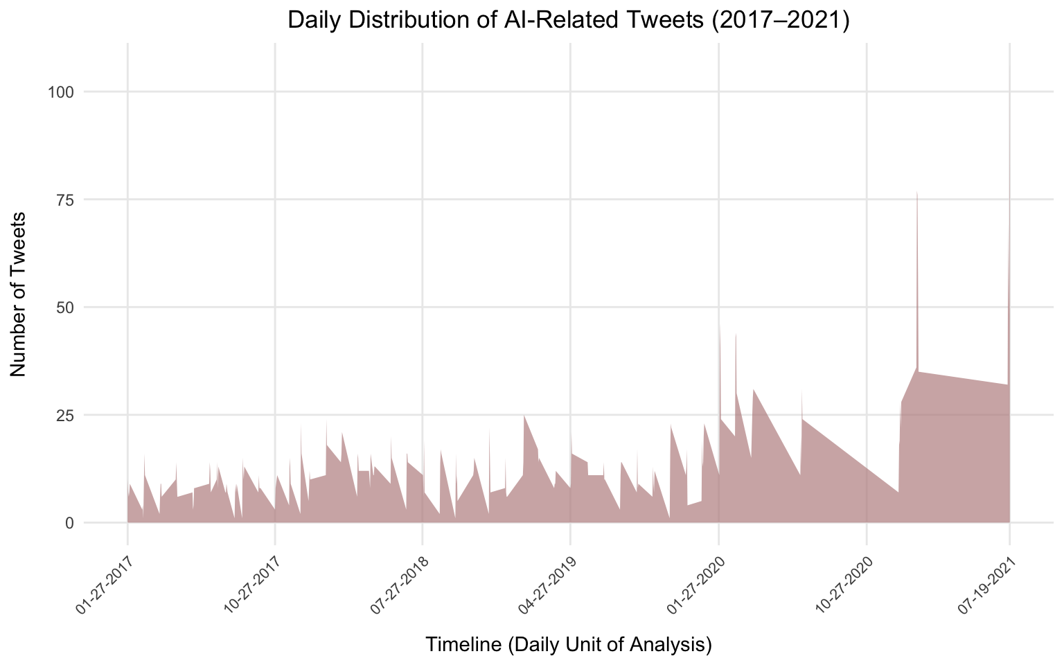
The date variable involved in this study is date_utc, derived from the original created_at variable and normalized to UTC (see Appendix for the conversion process). It ranges from January 27th, 2017, to July 19th, 2021, covering a total time span of 5 years (1,634 days).

The unit of analysis over time in this study is each day. Figure 1 shows the daily distribution of tweets, where the x-axis displays the time range of the dataset (January 27th, 2017, to July 19th, 2021) and the y-axis represents the counts of observed tweets by day. Overall, tweet volume remained relatively low and stable in the earlier years of the dataset, generally fluctuating between 0 and 20 tweets per day, before showing a notable increase in activity around 2020–2021, with several prominent spikes, including one approaching 100 tweets in a single day, suggesting a growing public interest in AI-related discourse toward the end of the observation period.

Code

cat("Date Range (yyyy-mm-dd):\n",
    as.character(range(data$date_utc)[1]), "to",
    as.character(range(data$date_utc)[2]), "\n")
max(data$date_utc) - min(data$date_utc)

Date Range (yyyy-mm-dd):
 2017-01-27 to 2021-07-19 
Time difference of 1634 days

Code

daily_count <- data |>
  count(date_utc)

min_date <- min(daily_count$date_utc)
max_date <- max(daily_count$date_utc)
# include both endpoints explicitly 
# so the axis always shows actual start/end dates
x_breaks <- sort(unique(c(min_date, seq(min_date, max_date, by = "9 months"), max_date)))

ggplot(daily_count, aes(x = date_utc, y = n)) +
  geom_area(fill = "rosybrown", alpha = 0.7) +
  scale_x_date(breaks = x_breaks, date_labels = "%m-%d-%Y") +
  labs(
    title = "Daily Distribution of AI-Related Tweets (2017–2021)",
    x = "Timeline (Daily Unit of Analysis)",
    y = "Number of Tweets"
  ) +
  theme_minimal() +
  theme(
    axis.text.x  = element_text(angle = 45, hjust = 1, size = 8),
    axis.title.x = element_text(margin = margin(t = 10)),
    axis.title.y = element_text(margin = margin(r = 10)),
    panel.grid.minor = element_blank(),
    plot.title = element_text(hjust = 0.5)
  )

Figure 1: Daily Distribution of AI-Related Tweets (2017–2021)

2.6 Text Variables

There are three textual variables involved in this study: text, hashtags, and cashtags.

2.6.1 Text

The text variable contains the unique textual content of each tweet, with no missing values (NAs) nor empty content (empty string ""), with a sample size of 3,000. The number of unique values in the text variable is 2,995. For example, "Brands Can't Afford to Underestimate the Power of Artificial Intelligence, OMD's Retail Revolution https://t.co/l1hSywqKgM #ai #ml #dl" is one of the values.

Code

cat("Number of Empty Tweets:", sum(data$text == ""), "\n")
cat("Number of Unique Tweets:", length(unique(data$text)), "\n\n")
cat("First 6 Unique Tweets:\n")
head(unique(data$text))

Number of Empty Tweets: 0 
Number of Unique Tweets: 2995 

First 6 Unique Tweets:
[1] "Brands Can’t Afford to Underestimate the Power of Artificial Intelligence, OMD’s Retail Revolution  https://t.co/l1hSywqKgM #ai #ml #dl"                    
[2] "NASA : One of our planet’s few exposed lava lakes is changing, and artificial intelligence…  https://t.co/h7Lp70dYlv)  https://t.co/JFljeXzLE0"             
[3] "Artificial intelligence to be showcased in Guangzhou  - Business -  https://t.co/Qk6gmORE4m  https://t.co/NsuAjIJiAo #ai #ml #dl"                           
[4] "Artificial Intelligence: Implications On Marketing, Analytics, And You  https://t.co/v8p1metjJE via @avinash via @avinash  https://t.co/SojmDRiXk6"         
[5] "#ArtificialIntelligence #AI Automation high on employers' agenda as skills gaps set to bite - CIPD (blog)  https://t.co/mtAfFTvA16  https://t.co/SNKDxkSUeT"
[6] "Surden on Values Embedded in Legal Artificial Intelligence @HarrySurden  https://t.co/vBkBoWU1Nz"

2.6.2 Hashtags

The hashtags is another textual variable. It contains lists of lowercase hashtags starting with the # symbol in each tweet (all hashtags from the original tweets were converted to lowercase), with no missing values (NAs). Specifically, it contains 2,059 non-empty values (i.e., 2,059 observations contain one or more hashtags), where there are 1,539 non-empty unique values (excluding "[]"). For instance, "['ai', 'ml', 'dl']" and "['artificialintelligence', 'ai']" are two of the values.

In addition, as each tweet can contain multiple hashtags, the values are separated into single hashtags to gain more nuanced insights (see Appendix for the separation process). As observed, there are 2,382 non-empty unique single hashtags. For example, "ai" and "ml" are two of the unique single hashtags.

Code

# count non-empty and unique hashtag values
unique_hashtags <- data |>
  filter(hashtags != "[]") |>
  select(hashtags) |>
  count(hashtags)

cat("Number of Non-empty Hashtags:", sum(data$hashtags != "[]"), "\n")
cat("Number of Unique Non-empty Hashtags:", nrow(unique_hashtags), "\n\n")
cat("First 6 Unique Hashtags:\n")
head(unique(data$hashtags))

Number of Non-empty Hashtags: 2059 
Number of Unique Non-empty Hashtags: 1539 

First 6 Unique Hashtags:
[1] "['ai', 'ml', 'dl']"                                  
[2] "[]"                                                  
[3] "['artificialintelligence', 'ai']"                    
[4] "['summer', 'artificialintelligence', 'ai']"          
[5] "['artificialintelligence', 'ai', 'nlp', 'ecommerce']"
[6] "['ai']"

Code

# find unique single hashtags
single_hashtags <- data |>
  mutate(single_hashtags = str_remove_all(hashtags, "[\\[\\]']")) |>
  separate_rows(single_hashtags, sep = ",\\s*") |>
  filter(single_hashtags != "") |>
  count(single_hashtags)

cat("Number of Non-empty Unique Single Hashtags:", nrow(single_hashtags), "\n\n")
cat("First 6 Non-empty Unique Single Hashtags:\n")
head(unique(single_hashtags$single_hashtags))

Number of Non-empty Unique Single Hashtags: 2382 

First 6 Non-empty Unique Single Hashtags:
[1] "004nino"         "100daysofcod"    "100daysofcode"   "100daysofmlcode"
[5] "10xgrowth"       "1trendstoday"

2.6.3 Cashtags

Likewise, the cashtags variable contains lists of lowercase cashtags in each tweet, which are clickable financial ticker symbols on Twitter (now X), formed by prefixing a stock or cryptocurrency abbreviation with the $ sign. There are no missing values (NAs), 22 non-empty values (i.e., 22 observations contain one or more cashtags), and 18 non-empty unique values. For example, "['aieq', 'bikr']" and "['blk']" are two of the values. Additionally, there are 23 non-empty unique single cashtags in total, such as "ark", "blk", and "btc".

Code

# count non-empty and unique cashtag values
unique_cashtags <- data |>
  filter(cashtags != "[]") |>
  select(cashtags) |>
  count(cashtags)

cat("Number of Non-empty Cashtags:", sum(data$cashtags != "[]"), "\n")
cat("Number of Non-empty Unique Cashtags:", nrow(unique_cashtags), "\n\n")
cat("First 6 Unique Cashtags:\n")
head(unique(data$cashtags))

Number of Non-empty Cashtags: 22 
Number of Non-empty Unique Cashtags: 18 

First 6 Unique Cashtags:
[1] "[]"               "['v']"            "['blk']"          "['infy']"        
[5] "['aieq', 'bikr']" "['qlys']"

Code

# strip list formatting and split into one row per cashtag
single_cashtags <- data |>
  mutate(single_cashtags = str_remove_all(cashtags, "[\\[\\]']")) |>
  separate_rows(single_cashtags, sep = ",\\s*") |>
  filter(single_cashtags != "") |>
  count(single_cashtags)

cat("Number of Non-empty Unique Single Cashtags:", nrow(single_cashtags), "\n\n")
cat("Head of Non-empty Unique Single Cashtags:\n")
head(unique(single_cashtags$single_cashtags))

Number of Non-empty Unique Single Cashtags: 23 

Head of Non-empty Unique Single Cashtags:
[1] "aieq" "ark"  "axxa" "bikr" "blk"  "btc"

2.7 Text Preparation

Text cleaning and tokenization are performed as a preprocessing step for subsequent analyses.

Code

# text cleaning
data <- data |>
  mutate(textBU = text) |>           # back up raw text before cleaning
  filter(!is.na(text)) |>
  mutate(
    text = textutils::HTMLdecode(text),           # decode HTML entities (e.g., &amp;)
    text = str_to_lower(text),                    # normalize to lowercase
    text = str_remove_all(text, "https?://\\S+"), # strip URLs
    text = str_remove_all(text, "\\d+"),          # strip digits
    text = str_remove_all(text, "[@]\\w+"),       # strip @mentions
    text = str_squish(text)                        # collapse extra whitespace
  ) |>
  mutate(
    tweet_index = row_number(),           # sequential ID for joining
    nwords      = str_count(text, "\\w+") # word count after cleaning
  )

head(data$text)

[1] "brands can’t afford to underestimate the power of artificial intelligence, omd’s retail revolution #ai #ml #dl"
[2] "nasa : one of our planet’s few exposed lava lakes is changing, and artificial intelligence…"                   
[3] "artificial intelligence to be showcased in guangzhou - business - #ai #ml #dl"                                 
[4] "artificial intelligence: implications on marketing, analytics, and you via via"                                
[5] "#artificialintelligence #ai automation high on employers' agenda as skills gaps set to bite - cipd (blog)"     
[6] "surden on values embedded in legal artificial intelligence"

Code

# tokenize hashtags
hashtag_tokens <- data |>
  select(tweet_index, date_utc, hashtags) |>
  mutate(hashtag = str_remove_all(hashtags, "[\\[\\]']")) |>
  separate_rows(hashtag, sep = ",\\s*") |>
  filter(hashtag != "")

# tokenize cashtags
cashtag_tokens <- data |>
  select(tweet_index, date_utc, cashtags) |>
  mutate(cashtag = str_remove_all(cashtags, "[\\[\\]']")) |>
  separate_rows(cashtag, sep = ",\\s*") |>
  filter(cashtag != "")

# tweet-level tag features
tag_features <- data |>
  select(tweet_index, date_utc, likes_count, replies_count, retweets_count) |>
  left_join(
    hashtag_tokens |> count(tweet_index, name = "n_hashtag"),
    by = "tweet_index"
  ) |>
  left_join(
    cashtag_tokens |> count(tweet_index, name = "n_cashtag"),
    by = "tweet_index"
  ) |>
  mutate(
    n_hashtag   = replace_na(n_hashtag, 0L),
    n_cashtag   = replace_na(n_cashtag, 0L),
    has_hashtag = n_hashtag > 0,
    has_cashtag = n_cashtag > 0,
    year        = year(date_utc)
  )

tag_features |>
  select(tweet_index, n_hashtag, n_cashtag, has_hashtag, has_cashtag) |>
  head()

# A tibble: 6 × 5
  tweet_index n_hashtag n_cashtag has_hashtag has_cashtag
        <int>     <int>     <int> <lgl>       <lgl>      
1           1         3         0 TRUE        FALSE      
2           2         0         0 FALSE       FALSE      
3           3         3         0 TRUE        FALSE      
4           4         0         0 FALSE       FALSE      
5           5         2         0 TRUE        FALSE      
6           6         0         0 FALSE       FALSE

3 Methods

3.1 Statistical Methods

Prior to model estimation, correlation analysis is conducted as an exploratory step to examine the pairwise relationships between thematic features, sentiment scores, and user engagement metrics. This preliminary analysis helps identify potential associations and informs the selection of variables for subsequent modeling, while also providing an initial understanding of the direction and strength of relationships within the dataset.

In the meantime, this paper employs Generalized Linear Models (GLMs) to generate models to examine the relationship between variables. GLMs were chosen over simple linear regression due to the nature of the engagement data containing a preponderance of zero values, which is a distributional characteristic that standard linear models may not adequately handle. By accommodating non-normal response distributions, GLMs offer a more flexible and appropriate modeling approach for count-based social media engagement data.

3.2 Text-as-Data Methods

For text analysis, this paper draws on two complementary computational techniques. Latent Dirichlet Allocation (LDA) topic modeling, which is a widely used unsupervised machine learning technique, is applied to uncover potential thematic structures within the dataset, identifying the core subjects that characterized AI-related discourse. Meanwhile, sentiment analysis with lexicons, a natural language processing approach evaluating the emotional tone of textual data by leveraging predefined lexical resources to classify polarity (e.g., positive, negative, or neutral), is also employed to establish the overall emotional polarity and trends among tweets. In addition, Term Frequency-Inverse Document Frequency (TF-IDF) is used to track how the salience of key AI-related terms shifted from 2017 to 2021, offering a longitudinal perspective on lexical change as AI moved toward mainstream adoption.

These methods directly support the research questions investigating how identified themes and sentiments polarities are associated with user engagement, as Topic Modeling and Sentiment Analysis allow the study to identify underlying themes and sentiments, while TF-IDF provides a temporal perspective on the evolving trends of AI-related key terms across the dataset. Together, these techniques inform the subsequent inferential analysis, in which GLM provide insights into the predictive relationships between textual variables and engagement metrics statistically.

4 Results

4.1 LDA Topic Modeling

To identify the underlying thematic structure of AI-related tweets, LDA was applied to the preprocessed tweet corpus. After tokenization, tweets were filtered using a custom stopword list that removed general English stopwords, Twitter-specific terms (e.g., "rt", "tweet"), and the search keyword "artificial intelligence". A TF-IDF filter then retained only words appearing in more than 0.1% but fewer than 75% of all documents, reducing vocabulary noise while preserving informative terms. The resulting document-term matrix served as input to the LDA model, which was estimated with K = 5 topics using Gibbs sampling with 2,000 iterations and a 500-iteration burn-in period.

Code

# custom domain-specific stopwords
mystopwords <- c(
  stop_words$word,
  "comment", "post",
  "twitter", "tweet", "tweets",
  "rt", "retweet", "retweets",
  "artificial", "intelligence"
)
mystopwords <- tolower(unique(mystopwords))
cat("Total stopwords:", length(mystopwords), "\n")

# tokenize
tm_token_data <- data |>
  unnest_tokens(word, text) |>
  anti_join(data.frame(word = mystopwords)) |>
  mutate(nchar = nchar(word)) |>
  filter(nchar > 2) |>
  filter(!grepl("[0-9]{1}", word)) |>
  filter(!grepl("\\W", word))

cat("Total tokens:", nrow(tm_token_data), "\n")

Total stopwords: 738 
Total tokens: 27565

Code

n_docs_total <- n_distinct(tm_token_data$tweet_index)

# retain words in (0.1%, 75%) document frequency range
good_words <- tm_token_data |>
  count(tweet_index, word) |>
  group_by(word) |>
  summarise(doc_freq = n() / n_docs_total, .groups = "drop") |>
  filter(doc_freq < 0.75, doc_freq > 0.001)

tm_token_data_pruned <- tm_token_data |>
  inner_join(good_words, by = "word")

cat("Vocabulary after TF-IDF filter:", nrow(good_words), "words\n")
cat("Tokens after filter:", nrow(tm_token_data_pruned), "\n")

# document-term matrix
tweet_dtm <- tm_token_data_pruned |>
  count(tweet_index, word) |>
  cast_dtm(tweet_index, word, n)

cat("DTM:", nrow(tweet_dtm), "documents x", ncol(tweet_dtm), "terms\n")

Vocabulary after TF-IDF filter: 1800 words
Tokens after filter: 20112 
DTM: 2961 documents x 1800 terms

Code

set.seed(32)
lda_model <- LDA(
  tweet_dtm, k = 5, method = "Gibbs",
  control = list(seed = 32, iter = 2000, burnin = 500, verbose = 0)
)
# persist to disk so the object survives 
# chunk-cache invalidation and is usable externally
save(lda_model, file = "./lda_model_ai.RData")

Figure 2 displays the top 10 words by probability (beta) for each of the five topics, providing the basis for thematic interpretation. Based on the word distributions, the topics were labeled as follows: Topic 1 represents robotics and automation, with key terms such as robotics, automation, and robot; Topic 2 reflects technology, research, and financial markets, featuring words like blockchain, technology, research, market, and healthcare; Topic 3 captures data science, machine learning, and security, with terms including data, learning, machine, and security; Topic 4 represents business-oriented AI innovation, characterized by words like business, future, innovation, digital, and digitaltransformation; and Topic 5 emphasizes applied AI ecosystem vocabulary, including machinelearning, bigdata, datascience, iot, and deeplearning.

Code

lda_beta <- tidy(lda_model, matrix = "beta")

lda_beta |>
  group_by(topic) |>
  slice_max(beta, n = 10) |>
  ungroup() |>
  mutate(term = reorder_within(term, beta, topic)) |>
  ggplot(aes(beta, term, fill = factor(topic))) +
  geom_col(show.legend = FALSE) +
  facet_wrap(~topic, scales = "free") +
  scale_y_reordered() +
  labs(
    title = "Top 10 Words per LDA Topic (K = 5)",
    x = "Beta (Word Probability)", 
    y = NULL
  ) +
  theme_minimal() +
  theme(
    plot.title = element_text(hjust = 0.5)
  )

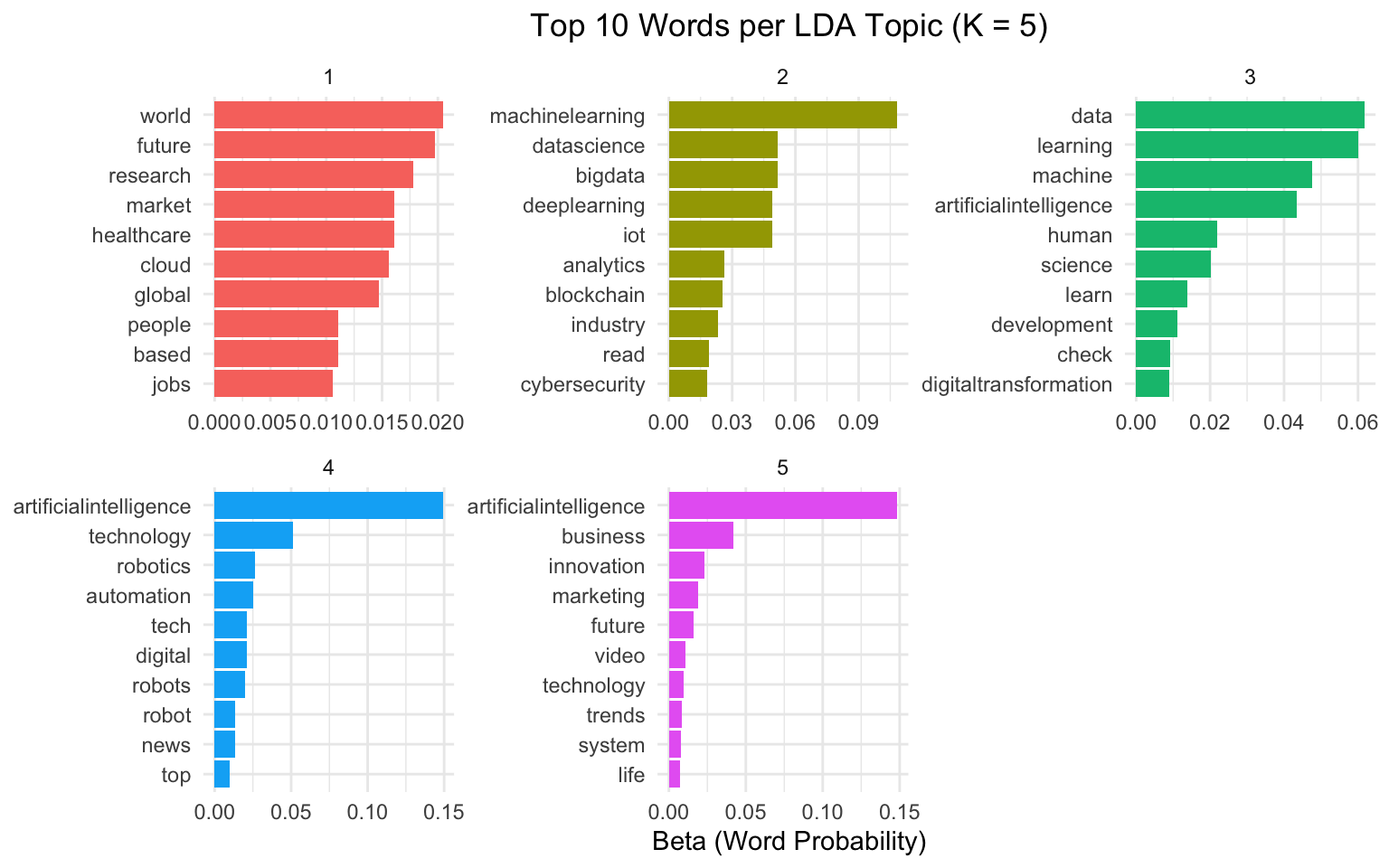
Figure 2: Top 10 Words per LDA Topic (K = 5)
*Note.* Bars represent word probability (beta) within each topic. Topics are labeled by their dominant semantic cluster.

Table 4 presents the distribution of dominant topics, which is the topic with the highest membership probability for each tweet, across the 3,000 sampled tweets. Topic 1 (robotics and automation) was the most prevalent, accounting for 28.4% of tweets, followed by Topic 2 (technology and markets, 23.3%), Topic 3 (data science and security, 19.0%), Topic 4 (business and innovation, 15.3%), and Topic 5 (AI ecosystem buzzwords, 14.0%). The distribution was moderately uneven, with Topics 1 and 2 together covering more than half of all tweets.

Code

# gamma matrix: document-topic probabilities
lda_gamma <- tidy(lda_model, matrix = "gamma")

# reshape wide and join with original data
gamma_wide <- lda_gamma |>
  mutate(tweet_index = as.integer(document)) |>
  select(-document) |>
  pivot_wider(names_from = topic, values_from = gamma, names_prefix = "topic_")

meta_theta_df <- data |>
  inner_join(gamma_wide, by = "tweet_index")

Code

# assign each tweet its dominant topic (highest gamma) and tabulate counts
dominant_dist <- lda_gamma |>
  group_by(document) |>
  slice_max(gamma, n = 1) |>
  ungroup() |>
  count(topic) |>
  mutate(pct = round(n / sum(n) * 100, 1))

knitr::kable(
  dominant_dist |>
    rename(
      Topic = topic,
      `Tweet Count` = n,
      `Percentage (%)` = pct
    ),
  align = c('c','c','c'),
  caption = "Distribution of Dominant LDA Topics Across Tweets"
)

Table 4: Distribution of Dominant LDA Topics Across Tweets

Topic	Tweet Count	Percentage (%)
1	865	20.7
2	779	18.7
3	837	20.1
4	833	20.0
5	855	20.5

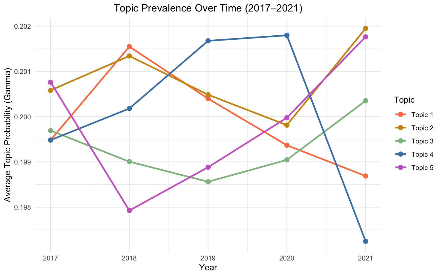
Figure 3 traces average topic probabilities (gamma) across years from 2017 to 2021. Notably, all five topics maintained average probabilities close to 0.20 throughout the study period, indicating a relatively stable thematic structure over time. Despite this overall stability, subtle directional shifts were present. Topic 4 (business and innovation) showed a modest upward trend from 2017 to 2021, while Topic 2 (technology and markets) declined slightly. Topic 5 (AI ecosystem buzzwords) also edged upward by 2021. These patterns suggest that while the broad thematic balance of AI discourse remained intact, business- and implementation-oriented language gradually gained somewhat greater prominence as AI moved toward mainstream adoption.

Code

# compute mean topic probability (gamma) per year for trend visualization
topics_by_year <- lda_gamma |>
  mutate(tweet_index = as.integer(document)) |>
  left_join(data |> select(tweet_index, date_utc), by = "tweet_index") |>
  mutate(year = year(date_utc)) |>
  group_by(year, topic) |>
  summarise(mean_gamma = mean(gamma), .groups = "drop")

ggplot(topics_by_year, aes(x = year, y = mean_gamma, color = factor(topic))) +
  geom_line(linewidth = 1) +
  geom_point(size = 2.5) +
  scale_x_continuous(breaks = 2017:2021) +
  scale_color_manual(
    values = c(
      "1" = "coral", "2" = "darkgoldenrod3", "3" = "darkseagreen",
      "4" = "steelblue", "5" = "orchid3"
    ),
    labels = paste("Topic", 1:5)
  ) +
  labs(
    title = "Topic Prevalence Over Time (2017–2021)",
    x = "Year", 
    y = "Average Topic Probability (Gamma)", 
    color = "Topic"
  ) +
  theme_minimal() +
  theme(
    plot.title = element_text(hjust = 0.5)
  )

Figure 3: Topic Prevalence Over Time (2017–2021)
*Note.* Lines represent mean gamma (topic membership probability) across all tweets in each year. All five topics remain close to 0.20 throughout the period, indicating thematic stability.

4.2 Hashtag and Cashtag Analysis

Hashtag and cashtag analysis complemented the topic model by examining the explicit user-generated labels that framed AI-related tweets. Table 5 summarizes the overall prevalence of hashtags and cashtags. Among the 3,000 sampled tweets, 2,059 (68.6%) contained at least one hashtag, with an average of 3.45 hashtags per tweet. By contrast, only 22 tweets (0.7%) contained any cashtag, with an average of just 0.01 per tweet. This large difference in frequency suggests that financial and market-oriented labeling through cashtags was marginal in this corpus, while hashtag use was both widespread and dense.

Code

# summarize hashtag and cashtag prevalence across the sample
tag_presence_table <- tibble(
  tag_type = c("Hashtag", "Cashtag"),
  tweets_with_tag = c(
    sum(tag_features$has_hashtag), sum(tag_features$has_cashtag)
  ),
  pct_with_tag    = round(tweets_with_tag / nrow(tag_features) * 100, 1),
  avg_tags_per_tweet = c(
    round(mean(tag_features$n_hashtag), 2),
    round(mean(tag_features$n_cashtag), 2)
  )
)

knitr::kable(
  tag_presence_table |>
    rename(
      `Tag Type`              = tag_type,
      `Tweets With Tag`       = tweets_with_tag,
      `Percent of Tweets (%)` = pct_with_tag,
      `Avg. Tags per Tweet`   = avg_tags_per_tweet
    ),
  align = 'c',
  caption = "Prevalence of Hashtags and Cashtags in the Sample"
)

Table 5: Prevalence of Hashtags and Cashtags in the Sample

Tag Type	Tweets With Tag	Percent of Tweets (%)	Avg. Tags per Tweet
Hashtag	2059	68.6	3.45
Cashtag	22	0.7	0.01

Table 6 and Figure 4 display the 15 most frequently used hashtags across the full 2017–2021 sample. The top three were #artificialintelligence (1,427 uses), #ai (1,094 uses), and #machinelearning (483 uses), followed by #bigdata, #datascience, #deeplearning, #iot, and #ml. This ranking indicates that AI tweets were predominantly framed through technical and industry labels rather than through social, ethical, or political categories.

Code

# count and rank all single hashtags; keep top 15
top_hashtags <- hashtag_tokens |>
  count(hashtag, sort = TRUE) |>
  slice_max(n, n = 15)

knitr::kable(
  top_hashtags |> rename(Hashtag = hashtag, Frequency = n),
  align = 'c',
  caption = "Most Frequent Hashtags in AI-Related Tweets (2017–2021)"
)

Table 6: Most Frequent Hashtags in AI-Related Tweets (2017–2021)

Hashtag	Frequency
artificialintelligence	1427
ai	1094
machinelearning	483
bigdata	230
datascience	229
deeplearning	218
iot	189
ml	184
technology	166
tech	111
robotics	99
analytics	88
blockchain	85
innovation	76
automation	75

Code

# horizontal bar chart of the 15 most frequent hashtags
top_hashtags |>
  mutate(hashtag = reorder(hashtag, n)) |>
  ggplot(aes(x = n, y = hashtag)) +
  geom_col(fill = "darkcyan", alpha = 0.8) +
  labs(
    title = "Top 15 Hashtags in AI-Related Tweets",
    x = "Frequency", y = NULL
  ) +
  theme_minimal() +
  theme(
    plot.title = element_text(hjust = 0.5)
  )

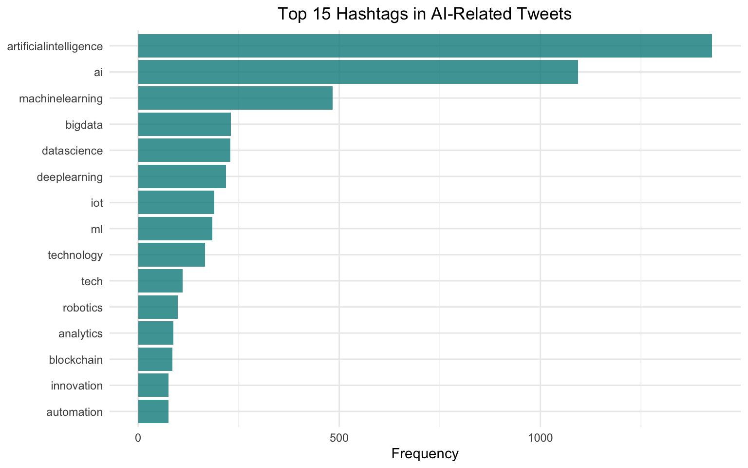
Figure 4: Top 15 Hashtags in AI-Related Tweets
*Note.* Bars show overall frequency across the 2017–2021 sample. Broad AI labels (#artificialintelligence, #ai) dominate, followed by applied technical subfield terms.

Table 7 presents the top five hashtags by year. #artificialintelligence and #ai remained the top two in every year from 2017 to 2021. However, the third through fifth positions shifted over time: in 2017 and 2018, #bigdata and #iot appeared prominently, while by 2020 and 2021, #datascience and #deeplearning replaced them. The count of #machinelearning grew steadily, from 47 uses in 2017 to 127 in 2021. Figure 5 shows the share trends for the eight most commonly used hashtags, visually confirming the persistence of general AI labels alongside the rising prominence of applied technical subfields.

Code

# count hashtags per year and keep the top 5 per year
top_hashtags_year <- hashtag_tokens |>
  mutate(year = year(date_utc)) |>
  count(year, hashtag, sort = TRUE) |>
  group_by(year) |>
  slice_max(n, n = 5, with_ties = FALSE) |>
  ungroup()

knitr::kable(
  top_hashtags_year |> rename(Year = year, Hashtag = hashtag, Frequency = n),
  align = 'c',
  caption = "Top Five Hashtags by Year (2017–2021)"
)

Table 7: Top Five Hashtags by Year (2017–2021)

Year	Hashtag	Frequency
2017	artificialintelligence	226
2017	ai	214
2017	machinelearning	47
2017	bigdata	38
2017	iot	34
2018	artificialintelligence	231
2018	ai	215
2018	machinelearning	76
2018	bigdata	49
2018	iot	43
2019	artificialintelligence	316
2019	ai	229
2019	machinelearning	120
2019	bigdata	53
2019	datascience	52
2020	artificialintelligence	335
2020	ai	217
2020	machinelearning	113
2020	datascience	61
2020	deeplearning	50
2021	artificialintelligence	319
2021	ai	219
2021	machinelearning	127
2021	datascience	77
2021	deeplearning	64

Code

# identify the 8 most common hashtags overall
focus_hashtags <- hashtag_tokens |>
  count(hashtag, sort = TRUE) |>
  slice_max(n, n = 8, with_ties = FALSE) |>
  pull(hashtag)

# compute each hashtag's share of uses within each year
hashtag_trends <- hashtag_tokens |>
  mutate(year = year(date_utc)) |>
  filter(hashtag %in% focus_hashtags) |>
  count(year, hashtag) |>
  group_by(year) |>
  mutate(pct_year = n / sum(n)) |>
  ungroup()

ggplot(hashtag_trends, aes(x = year, y = pct_year, color = hashtag)) +
  geom_line(linewidth = 1) +
  geom_point(size = 2) +
  scale_x_continuous(breaks = 2017:2021) +
  scale_y_continuous(labels = percent_format(accuracy = 1)) +
  labs(
    title = "Top Hashtag Shares by Year",
    x = "Year", 
    y = "Share of Hashtag Uses", 
    color = "Hashtag"
  ) +
  theme_minimal() +
  theme(
    plot.title = element_text(hjust = 0.5)
  )

Figure 5: Top Hashtag Shares by Year
*Note.* Lines show each hashtag’s share among the eight most common hashtags in each year. General AI labels maintain dominance while technical subfield terms gradually increase.

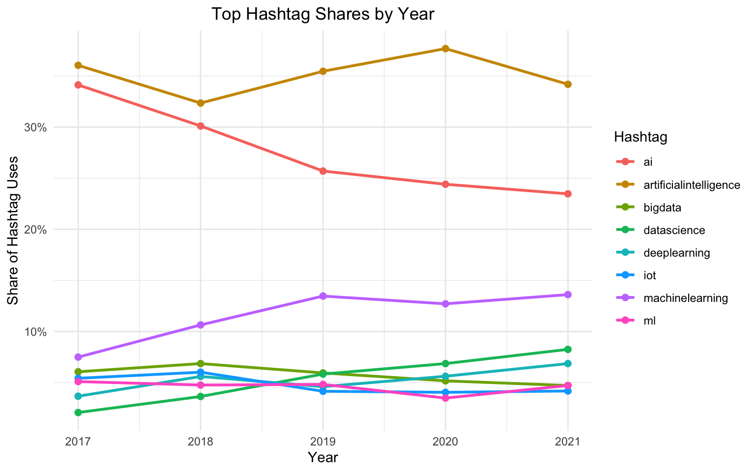
Table 8 presents the most frequently used cashtags. The top cashtags were $btc (4 uses), $btcusd (3 uses), and $v (3 uses), with nearly all others appearing only once. The very low frequency of cashtags indicates that market- and investment-oriented discourse about AI occupied a very small niche in this corpus, and cashtags are better understood as occasional markers of crypto- or finance-adjacent AI talk rather than a major framing device.

Code

# count and rank cashtag frequency; keep top 5
top_cashtags <- cashtag_tokens |>
  count(cashtag, sort = TRUE) |>
  slice_max(n, n = 5)

knitr::kable(
  top_cashtags |> rename(Cashtag = cashtag, Frequency = n),
  align = 'c',
  caption = "Most Frequent Cashtags in AI-Related Tweets (2017–2021)"
)

Table 8: Most Frequent Cashtags in AI-Related Tweets (2017–2021)

Cashtag	Frequency
btc	4
btcusd	3
v	3
aieq	1
ark	1
axxa	1
bikr	1
blk	1
eth	1
fcac	1
goog	1
gtch	1
icr	1
infy	1
ipod	1
ipof	1
jar	1
mark	1
phun	1
qlys	1
svfau	1
vrx	1
vsby	1

4.3 Sentiment Analysis

4.3.1 Comparison of Sentiment Lexicons

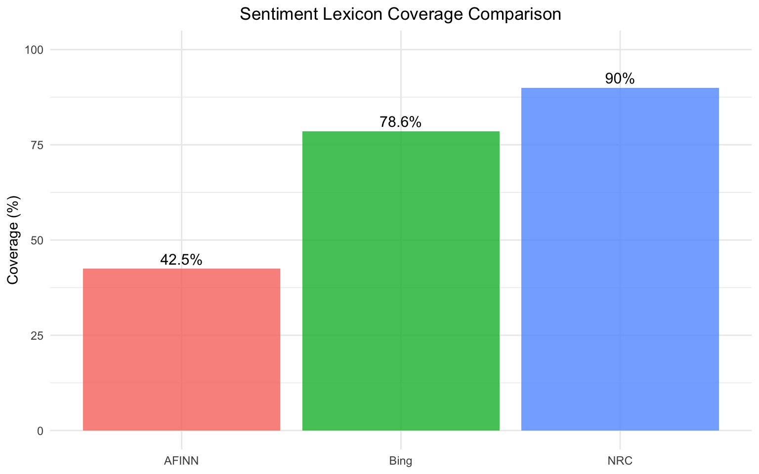
Sentiment analysis was conducted using three established dictionary lexicons: AFINN, Bing, and NRC. Table 9 summarizes their coverage in the dataset. NRC achieved the broadest coverage at 90.0% of tweets scored, followed by Bing at 78.6%, and AFINN at 42.5%. Figure 6 displays these differences visually. Despite its lower coverage, AFINN was selected as the primary sentiment measure for three reasons. First, AFINN provides a continuous intensity scale (–5 to +5) that captures the degree of positive or negative sentiment, making it directly suitable for regression modeling. Second, among the 1,130 tweets scored by all three lexicons, AFINN correlated strongly with Bing (r = .664) and moderately with NRC (r = .510), while Bing and NRC correlated at r = .528, confirming that all three measures captured a consistent underlying signal. Third, the additional tweets scored by NRC did not justify the increased interpretive complexity of a categorical emotion framework for the purposes of this analysis.

Code

# tokenize and remove stopwords for sentiment analysis
sa_token_data <- data |>
  unnest_tokens(word, text) |>
  anti_join(stop_words, by = "word") |>
  mutate(nchar_w = nchar(word))

cat("Total tokens:", nrow(sa_token_data), "\n")
cat("Unique tokens:", n_distinct(sa_token_data$word), "\n")
cat("Avg tokens per tweet:",
    round(nrow(sa_token_data) / n_distinct(sa_token_data$tweet_index), 1), "\n")

Total tokens: 34076 
Unique tokens: 8236 
Avg tokens per tweet: 11.4

Code

# AFINN: numeric scores from -5 (very negative) to +5 (very positive)
afinn_scores <- sa_token_data |>
  inner_join(get_sentiments("afinn"), by = "word") |>
  group_by(tweet_index) |>
  summarise(
    sentiment_afinn = sum(value),
    n_afinn_words   = n(),
    avg_afinn       = mean(value),
    .groups = "drop"
  )

afinn_coverage     <- nrow(afinn_scores)
afinn_coverage_pct <- round(afinn_coverage / nrow(data) * 100, 1)
cat("AFINN coverage:", afinn_coverage, "tweets (", afinn_coverage_pct, "% )\n")

AFINN coverage: 1275 tweets ( 42.5 % )

Code

# Bing: binary positive / negative classification
bing_scores <- sa_token_data |>
  inner_join(get_sentiments("bing"), by = "word") |>
  group_by(tweet_index) |>
  summarise(
    n_positive     = sum(sentiment == "positive"),
    n_negative     = sum(sentiment == "negative"),
    n_bing_words   = n(),
    sentiment_bing = n_positive - n_negative,
    .groups = "drop"
  )

bing_coverage     <- nrow(bing_scores)
bing_coverage_pct <- round(bing_coverage / nrow(data) * 100, 1)
cat("Bing coverage:", bing_coverage, "tweets (", bing_coverage_pct, "%)\n")

Bing coverage: 2359 tweets ( 78.6 %)

Code

# NRC: 8 basic emotions + positive / negative
nrc_raw <- sa_token_data |>
  inner_join(get_sentiments("nrc"), by = "word")

nrc_scores <- nrc_raw |>
  group_by(tweet_index, sentiment) |>
  summarise(n = n(), .groups = "drop") |>
  pivot_wider(names_from = sentiment, values_from = n, values_fill = 0) |>
  mutate(sentiment_nrc = positive - negative)

nrc_coverage     <- nrow(nrc_scores)
nrc_coverage_pct <- round(nrc_coverage / nrow(data) * 100, 1)
cat("NRC coverage:", nrc_coverage, "tweets (", nrc_coverage_pct, "%)\n")

NRC coverage: 2700 tweets ( 90 %)

Code

# assemble pre-computed coverage counts into a comparison table
coverage_df <- data.frame(
  lexicon       = c("AFINN", "Bing", "NRC"),
  tweets_scored = c(afinn_coverage, bing_coverage, nrc_coverage),
  coverage_pct  = c(afinn_coverage_pct, bing_coverage_pct, nrc_coverage_pct)
)

knitr::kable(
  coverage_df |>
    rename(
      Lexicon         = lexicon,
      `Tweets Scored` = tweets_scored,
      `Coverage (%)`  = coverage_pct
    ),
  align = 'c',
  caption = "Coverage of Sentiment Lexicons Across the Tweet Sample"
)

Table 9: Coverage of Sentiment Lexicons Across the Tweet Sample

Lexicon	Tweets Scored	Coverage (%)
AFINN	1275	42.5
Bing	2359	78.6
NRC	2700	90.0

Code

# bar chart comparing tweet coverage (%) across the three lexicons
ggplot(coverage_df, aes(x = lexicon, y = coverage_pct, fill = lexicon)) +
  geom_col(alpha = 0.8) +
  geom_text(aes(label = paste0(coverage_pct, "%")), vjust = -0.4, size = 4) +
  ylim(0, 100) +
  labs(
    title = "Sentiment Lexicon Coverage Comparison",
    x = NULL, 
    y = "Coverage (%)"
  ) +
  theme_minimal() +
  theme(
    legend.position = "none",
    plot.title = element_text(hjust = 0.5)
  )

Figure 6: Sentiment Lexicon Coverage Comparison
*Note.* Bars represent the percentage of the 3,000 tweets that received a sentiment score from each lexicon. NRC achieves the widest coverage; AFINN covers a smaller share but provides continuous intensity scores.

Code

# correlations among tweets scored by all three lexicons
sentiment_cmp <- data |>
  select(tweet_index) |>
  left_join(afinn_scores |> select(tweet_index, sentiment_afinn), by = "tweet_index") |>
  left_join(bing_scores  |> select(tweet_index, sentiment_bing),  by = "tweet_index") |>
  left_join(nrc_scores   |> select(tweet_index, sentiment_nrc),   by = "tweet_index")

complete_cmp <- sentiment_cmp |>
  filter(!is.na(sentiment_afinn), !is.na(sentiment_bing), !is.na(sentiment_nrc))

cat("Tweets scored by all three lexicons:", nrow(complete_cmp), "\n")
cat("AFINN vs Bing: r =",
    round(cor(complete_cmp$sentiment_afinn, complete_cmp$sentiment_bing), 3), "\n")
cat("AFINN vs NRC:  r =",
    round(cor(complete_cmp$sentiment_afinn, complete_cmp$sentiment_nrc), 3), "\n")
cat("Bing  vs NRC:  r =",
    round(cor(complete_cmp$sentiment_bing,  complete_cmp$sentiment_nrc), 3), "\n")

Tweets scored by all three lexicons: 1130 
AFINN vs Bing: r = 0.665 
AFINN vs NRC:  r = 0.509 
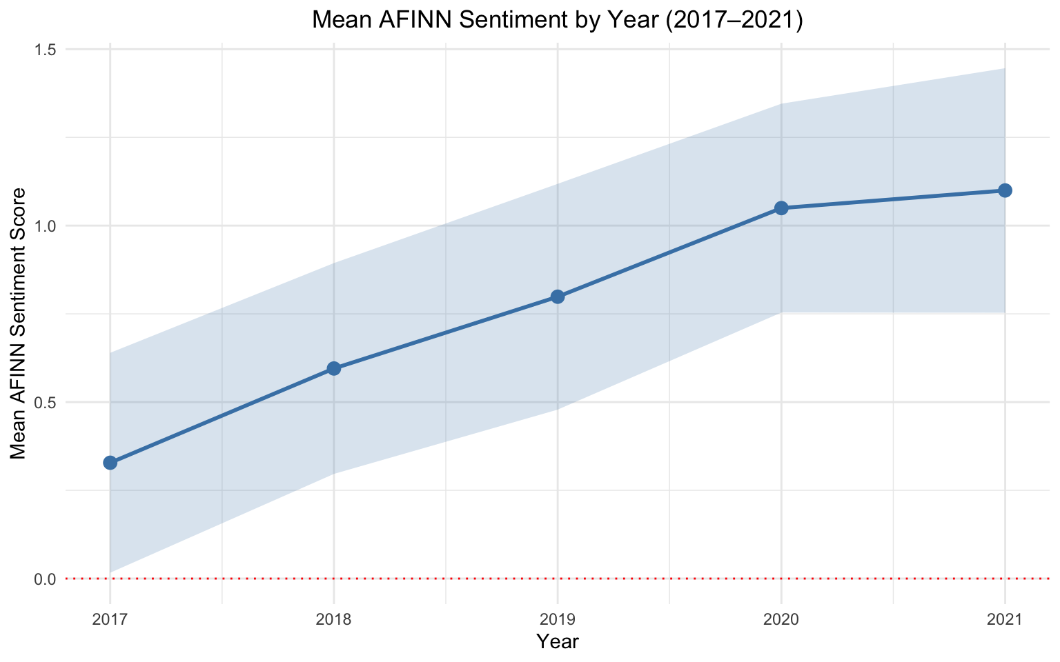
Bing  vs NRC:  r = 0.529

4.3.2 Temporal Trends in Sentiment

Among the 1,275 tweets that received AFINN scores, overall sentiment in the corpus was slightly positive (M = 0.81, Median = 1, range: -18 to 12). Table 10 and Figure 7 present mean AFINN scores by year with 95% confidence intervals. A clear upward trend is visible: mean sentiment increased from 0.33 in 2017 to 0.60 in 2018, 0.80 in 2019, 1.05 in 2020, and 1.11 in 2021. The 95% confidence intervals indicate that this upward movement became increasingly stable in later years. This pattern is consistent with the growing normalization of AI as a practical and promising technology, where public discourse shifted toward greater optimism about AI’s applications and societal benefits.

Code

# attach AFINN scores to data and propagate to meta_theta_df
data <- data |>
  left_join(afinn_scores |> select(tweet_index, sentiment_afinn), by = "tweet_index") |>
  mutate(sentiment_norm = sentiment_afinn / nwords)

meta_theta_df <- meta_theta_df |>
  left_join(afinn_scores |> select(tweet_index, sentiment_afinn), by = "tweet_index")

n_scored <- sum(!is.na(data$sentiment_afinn))
cat("Tweets with AFINN scores:", n_scored,
    paste0("(", round(n_scored / nrow(data) * 100, 1), "%)"), "\n")
summary(data$sentiment_afinn)

Tweets with AFINN scores: 1275 (42.5%) 
    Min.  1st Qu.   Median     Mean  3rd Qu.     Max.     NA's 
-18.0000  -1.0000   1.0000   0.8071   2.0000  12.0000     1725

Code

# yearly mean AFINN scores with standard errors and 95% CIs
sentiment_by_year <- data |>
  filter(!is.na(sentiment_afinn)) |>
  mutate(year = year(date_utc)) |>
  group_by(year) |>
  summarise(
    n         = n(),
    mean_sent = mean(sentiment_afinn),
    se_sent   = sd(sentiment_afinn) / sqrt(n),
    .groups   = "drop"
  ) |>
  mutate(
    ci_low  = mean_sent - 1.96 * se_sent,
    ci_high = mean_sent + 1.96 * se_sent
  )

knitr::kable(
  sentiment_by_year |>
    rename(
      Year = year, `Tweets Scored` = n, `Mean Sentiment` = mean_sent,
      SE = se_sent, `95% CI Low` = ci_low, `95% CI High` = ci_high
    ),
  align = 'c',
  caption = "Mean AFINN Sentiment Score by Year with 95% Confidence Intervals",
  digits  = 3
)

Table 10: Mean AFINN Sentiment Score by Year with 95% Confidence Intervals

Year	Tweets Scored	Mean Sentiment	SE	95% CI Low	95% CI High
2017	192	0.328	0.159	0.017	0.640
2018	252	0.595	0.152	0.297	0.894
2019	278	0.799	0.163	0.479	1.118
2020	282	1.050	0.151	0.754	1.345
2021	271	1.100	0.177	0.753	1.446

Code

# line + confidence ribbon showing mean AFINN sentiment trend from 2017 to 2021
ggplot(sentiment_by_year, aes(x = year, y = mean_sent)) +
  geom_ribbon(aes(ymin = ci_low, ymax = ci_high), alpha = 0.2, fill = "steelblue") +
  geom_line(color = "steelblue", linewidth = 1) +
  geom_point(color = "steelblue", size = 3) +
  geom_hline(yintercept = 0, linetype = "dotted", color = "red") +
  scale_x_continuous(breaks = 2017:2021) +
  labs(
    title = "Mean AFINN Sentiment by Year (2017–2021)",
    x = "Year", 
    y = "Mean AFINN Sentiment Score"
  ) +
  theme_minimal() +
  theme(
    plot.title = element_text(hjust = 0.5)
  )

Figure 7: Mean AFINN Sentiment by Year (2017–2021)
*Note.* Points and line show yearly means; the ribbon represents the 95% confidence interval. The dashed horizontal line marks a score of zero (neutral). Sentiment increased consistently from 2017 to 2021.

4.3.3 Topic–Sentiment Relationship

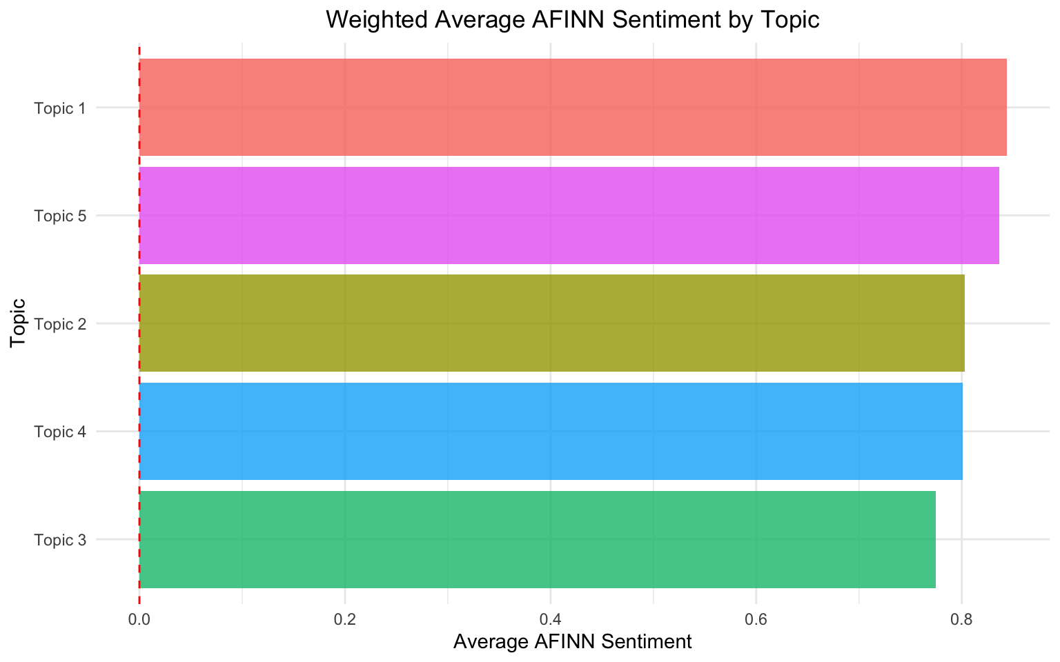
To examine whether discourse topics were associated with different emotional tones, average AFINN sentiment was computed for each topic using gamma-weighted scores, where each tweet’s contribution to a topic’s average sentiment was proportional to its membership probability in that topic. Figure 8 presents these weighted averages. Sentiment scores were very similar across all five topics, ranging from 0.79 (Topic 5, AI ecosystem buzzwords) to 0.84 (Topic 4, business and innovation). A weighted linear regression model predicting sentiment from topic membership found no statistically significant differences relative to Topic 1 for any other topic (all p > .80). This result shows that in this corpus, emotional tone did not vary meaningfully across thematic clusters; rather, sentiment varied more consistently over time than across topics.

Code

# compute weighted sentiment per topic
meta_theta_df <- meta_theta_df |>
  filter(!is.na(sentiment_afinn)) |>
  mutate(
    wt_sent_t1 = sentiment_afinn * topic_1,
    wt_sent_t2 = sentiment_afinn * topic_2,
    wt_sent_t3 = sentiment_afinn * topic_3,
    wt_sent_t4 = sentiment_afinn * topic_4,
    wt_sent_t5 = sentiment_afinn * topic_5
  )

topic_sent_avg <- tibble(
  topic = 1:5,
  total_weighted = c(
    sum(meta_theta_df$wt_sent_t1), sum(meta_theta_df$wt_sent_t2),
    sum(meta_theta_df$wt_sent_t3), sum(meta_theta_df$wt_sent_t4),
    sum(meta_theta_df$wt_sent_t5)
  ),
  gamma_mass = c(
    sum(meta_theta_df$topic_1), sum(meta_theta_df$topic_2),
    sum(meta_theta_df$topic_3), sum(meta_theta_df$topic_4),
    sum(meta_theta_df$topic_5)
  )
) |>
  mutate(
    avg_sentiment = total_weighted / gamma_mass,
    topic_label   = paste("Topic", topic)
  )

Code

# horizontal bar chart of gamma-weighted average AFINN sentiment per topic
ggplot(
  topic_sent_avg,
  aes(x = reorder(topic_label, avg_sentiment), y = avg_sentiment, fill = topic_label)
) +
  geom_col(alpha = 0.8) +
  geom_hline(yintercept = 0, linetype = "dashed", color = "red") +
  coord_flip() +
  labs(
    title = "Weighted Average AFINN Sentiment by Topic",
    x = "Topic", 
    y = "Average AFINN Sentiment"
  ) +
  theme_minimal() +
  theme(
    legend.position = "none", 
    plot.title = element_text(hjust = 0.5)
  )

Figure 8: Weighted Average AFINN Sentiment by Topic
*Note.* Bars represent the average sentiment score for each topic, weighted by gamma (topic membership probability). The dashed line marks neutral sentiment. Differences across topics are minimal and statistically non-significant.

Code

# weighted regression: sentiment ~ topic (verifies non-significant differences)
sentiment_topic_long <- meta_theta_df |>
  select(tweet_index, sentiment_afinn, starts_with("topic_")) |>
  pivot_longer(
    cols         = starts_with("topic_"),
    names_to     = "topic",
    values_to    = "gamma",
    names_prefix = "topic_"
  ) |>
  mutate(topic = factor(topic, levels = as.character(1:5)))

weighted_model <- lm(sentiment_afinn ~ topic, data = sentiment_topic_long, weights = gamma)
summary(weighted_model)


Call:
lm(formula = sentiment_afinn ~ topic, data = sentiment_topic_long, 
    weights = gamma)

Weighted Residuals:
    Min      1Q  Median      3Q     Max 
-9.6154 -0.8085  0.0898  0.5569  5.6288 

Coefficients:
             Estimate Std. Error t value Pr(>|t|)    
(Intercept)  0.843559   0.072602  11.619   <2e-16 ***
topic2      -0.040555   0.103362  -0.392    0.695    
topic3      -0.068844   0.103068  -0.668    0.504    
topic4      -0.042529   0.102899  -0.413    0.679    
topic5      -0.006947   0.102690  -0.068    0.946    
---
Signif. codes:  0 '***' 0.001 '**' 0.01 '*' 0.05 '.' 0.1 ' ' 1

Residual standard error: 1.163 on 6350 degrees of freedom
Multiple R-squared:  9.466e-05, Adjusted R-squared:  -0.0005352 
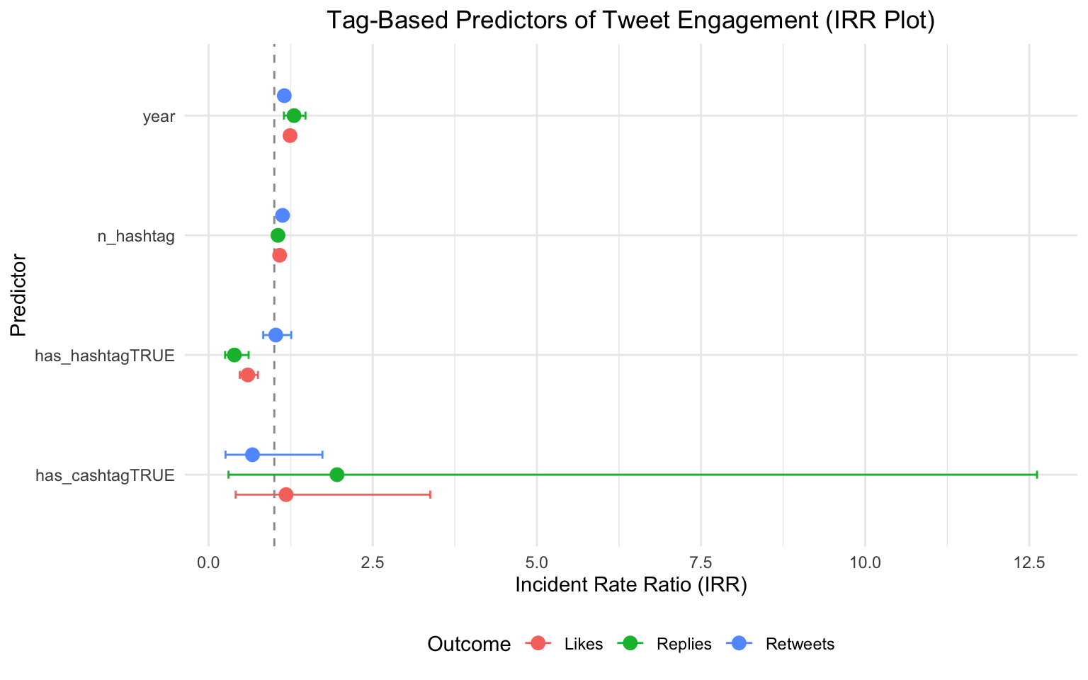
F-statistic: 0.1503 on 4 and 6350 DF,  p-value: 0.9629

4.4 Predictors of User Engagement

4.4.1 Hashtag and Cashtag Features

To examine whether content packaging was associated with engagement (RQ2), mean engagement metrics were first compared by tag presence (Table 11), and then three negative binomial GLMs were fitted predicting likes, replies, and retweets from hashtag presence, hashtag count, cashtag presence, and year (Table 12, Figure 9).

Descriptively, tweets containing hashtags received slightly higher mean likes (3.11 vs. 2.89) and notably higher mean retweets (2.86 vs. 1.23), though slightly fewer replies on average (0.12 vs. 0.19). Tweets with cashtags had higher mean values on all three metrics, but the number of cashtag-containing tweets was too small (n = 22) for reliable comparison.

Code

# compute mean engagement metrics by hashtag and cashtag presence
tag_engagement_summary <- tag_features |>
  summarise(
    likes_no_hashtag    = round(mean(likes_count[!has_hashtag]), 2),
    likes_hashtag       = round(mean(likes_count[has_hashtag]), 2),
    retweets_no_hashtag = round(mean(retweets_count[!has_hashtag]), 2),
    retweets_hashtag    = round(mean(retweets_count[has_hashtag]), 2),
    replies_no_hashtag  = round(mean(replies_count[!has_hashtag]), 2),
    replies_hashtag     = round(mean(replies_count[has_hashtag]), 2),
    likes_no_cashtag    = round(mean(likes_count[!has_cashtag]), 2),
    likes_cashtag       = round(mean(likes_count[has_cashtag]), 2),
    retweets_no_cashtag = round(mean(retweets_count[!has_cashtag]), 2),
    retweets_cashtag    = round(mean(retweets_count[has_cashtag]), 2),
    replies_no_cashtag  = round(mean(replies_count[!has_cashtag]), 2),
    replies_cashtag     = round(mean(replies_count[has_cashtag]), 2)
  )

knitr::kable(
  tibble(
    Condition       = c("No Hashtag", "Hashtag", "No Cashtag", "Cashtag"),
    `Mean Likes`    = c(tag_engagement_summary$likes_no_hashtag,
                        tag_engagement_summary$likes_hashtag,
                        tag_engagement_summary$likes_no_cashtag,
                        tag_engagement_summary$likes_cashtag),
    `Mean Replies`  = c(tag_engagement_summary$replies_no_hashtag,
                        tag_engagement_summary$replies_hashtag,
                        tag_engagement_summary$replies_no_cashtag,
                        tag_engagement_summary$replies_cashtag),
    `Mean Retweets` = c(tag_engagement_summary$retweets_no_hashtag,
                        tag_engagement_summary$retweets_hashtag,
                        tag_engagement_summary$retweets_no_cashtag,
                        tag_engagement_summary$retweets_cashtag)
  ),
  align = c('l', 'c', 'c', 'c'),
  caption = "Mean Engagement Metrics by Tag Presence"
)

Table 11: Mean Engagement Metrics by Tag Presence

Condition	Mean Likes	Mean Replies	Mean Retweets
No Hashtag	2.89	0.19	1.23
Hashtag	3.11	0.12	2.86
No Cashtag	3.04	0.14	2.35
Cashtag	4.05	0.23	2.41

Table 12 and Figure 9 present the exponentiated regression coefficients (incident rate ratios, IRRs) from the tag-based negative binomial models. The number of hashtags per tweet was a positive predictor of all three engagement outcomes: likes (IRR = 1.08, p < .001), replies (IRR = 1.06, p = .021), and retweets (IRR = 1.13, p < .001). By contrast, simply having any hashtag at all was a negative predictor for likes (IRR = 0.60, p < .001) and replies (IRR = 0.39, p < .001) once hashtag count was included in the model, and was not significant for retweets. This pattern reflects a compositional effect: tweets with only one or two hashtags do not benefit from the discoverability that rich hashtag networks provide, whereas tweets with many hashtags tend to attract more engagement across all metrics. Cashtag presence was not significantly associated with any engagement outcome.

Code

# fit negative binomial GLMs for each engagement metric using tag features
tag_glm_likes <- glm.nb(
  likes_count ~ has_hashtag + has_cashtag + n_hashtag + year,
  data = tag_features
)
tag_glm_replies <- glm.nb(
  replies_count ~ has_hashtag + has_cashtag + n_hashtag + year,
  data = tag_features
)
tag_glm_retweets <- glm.nb(
  retweets_count ~ has_hashtag + has_cashtag + n_hashtag + year,
  data = tag_features
)

tag_models <- list(Likes = tag_glm_likes, Replies = tag_glm_replies, Retweets = tag_glm_retweets)

tag_coef_all <- bind_rows(lapply(names(tag_models), function(nm) {
  tidy(tag_models[[nm]], exponentiate = TRUE) |>
    filter(term != "(Intercept)") |>
    mutate(
      # Wald CIs on the log-rate scale (delta method)
      # faster than profile-likelihood confint()
      conf.low  = estimate * exp(-1.96 * std.error),
      conf.high = estimate * exp( 1.96 * std.error),
      outcome   = nm
    )
}))

Code

# extract and format exponentiated coefficients (IRRs) from the tag GLMs
knitr::kable(
  tag_coef_all |>
    select(outcome, term, estimate, conf.low, conf.high, p.value) |>
    mutate(
      term = recode(term,
        "has_hashtagTRUE" = "Has Hashtag",
        "has_cashtagTRUE" = "Has Cashtag",
        "n_hashtag"       = "Number of Hashtags",
        "year"            = "Year"
      ),
      outcome = factor(outcome, levels = c("Likes", "Replies", "Retweets"))
    ) |>
    rename(
      Outcome = outcome, Predictor = term, IRR = estimate,
      `95% CI Low` = conf.low, `95% CI High` = conf.high, `p` = p.value
    ),
  caption = "Negative Binomial GLMs: Tag Features Predicting User Engagement",
  align = c('l', 'l', 'c', 'c', 'c', 'c'),
  digits  = 3
)

Table 12: Negative Binomial GLMs: Tag Features Predicting User Engagement

Outcome	Predictor	IRR	95% CI Low	95% CI High	p
Likes	Has Hashtag	0.596	0.474	0.751	0.000
Likes	Has Cashtag	1.179	0.412	3.375	0.759
Likes	Number of Hashtags	1.081	1.055	1.108	0.000
Likes	Year	1.239	1.161	1.322	0.000
Replies	Has Hashtag	0.391	0.251	0.609	0.000
Replies	Has Cashtag	1.955	0.303	12.618	0.481
Replies	Number of Hashtags	1.056	1.008	1.106	0.021
Replies	Year	1.300	1.147	1.475	0.000
Retweets	Has Hashtag	1.023	0.832	1.258	0.832
Retweets	Has Cashtag	0.667	0.257	1.733	0.406
Retweets	Number of Hashtags	1.125	1.102	1.150	0.000
Retweets	Year	1.152	1.088	1.220	0.000

Code

# IRR dot plot with 95% CIs for tag-based engagement predictors
ggplot(tag_coef_all, aes(x = estimate, y = term, color = outcome)) +
  geom_vline(xintercept = 1, linetype = "dashed", color = "gray60") +
  geom_point(size = 3, position = position_dodge(0.5)) +
  geom_errorbarh(
    aes(xmin = conf.low, xmax = conf.high),
    height = 0.2, position = position_dodge(0.5)
  ) +
  labs(
    title = "Tag-Based Predictors of Tweet Engagement (IRR Plot)",
    x = "Incident Rate Ratio (IRR)", y = "Predictor", color = "Outcome"
  ) +
  theme_minimal() +
  theme(
    legend.position = "bottom", 
    plot.title = element_text(hjust = 0.5)
  )

Figure 9: Tag-Based Predictors of Tweet Engagement (IRR Plot)
*Note.* Points represent incident rate ratios (IRRs) and horizontal bars represent 95% confidence intervals. The dashed vertical line at IRR = 1 indicates no effect. IRR > 1 indicates a positive association with engagement.

4.4.2 Sentiment and Topic as Predictors

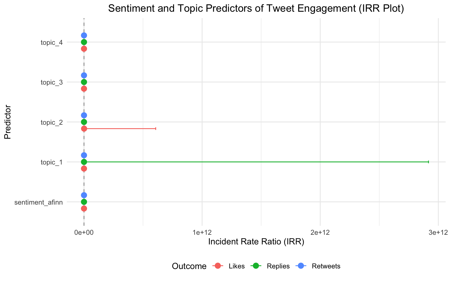
To directly test the associations between discourse characteristics and engagement, three negative binomial GLMs were fitted predicting likes, replies, and retweets from AFINN sentiment scores, LDA topic probabilities (Topics 1–4, with Topic 5 as the implicit baseline through the compositional constraint), and year fixed effects (Table 13, Figure 10).

AFINN sentiment was not a statistically significant predictor of any engagement outcome. Its IRR was 0.99 for likes (p = .676), 0.92 for replies (p = .081), and 0.98 for retweets (p = .383). This finding indicates that a more positive or more negative emotional tone alone did not reliably increase or decrease engagement once topic composition and year were taken into account.

By contrast, year was a consistent and substantial predictor of engagement. Relative to 2017, tweets from 2018 showed dramatically higher expected likes (IRR = 4.00) and replies (IRR = 8.23), and tweets from 2020 and 2021 also showed significantly higher likes and replies. Retweets were significantly higher in 2018 (IRR = 2.13) and 2021 (IRR = 2.12) relative to 2017. These large year effects suggest that the overall audience for AI content on Twitter grew substantially after 2017, leading to more engagement across the board regardless of the content’s tone.

Topic effects were present for some outcomes but should be interpreted carefully because LDA topic probabilities are compositional—increasing one topic’s probability necessarily reduces the others. Topic 2 showed a strong negative association with likes and retweets, while Topic 4 showed a strong positive association with replies. However, some estimated IRRs were extremely large or small, indicating instability likely due to near-collinearity among topic predictors. The most defensible interpretation is that business-innovation framing (Topic 4) may be associated with more conversational engagement, while certain technology-and-market content (Topic 2) may attract less passive amplification, but these conclusions require further testing with more robust specifications.

Code

# convert year to a factor so GLMs treat it as categorical fixed effects
glm_data <- meta_theta_df |>
  mutate(year = factor(year(date_utc)))

Code

# NB GLM: AFINN sentiment + LDA topic probabilities + year predicting likes
glm_likes <- glm.nb(
  likes_count ~ sentiment_afinn + topic_1 + topic_2 + topic_3 + topic_4 + year,
  data = glm_data
)
cat("=== Model: likes_count ===\n")
summary(glm_likes)

=== Model: likes_count ===

Call:
glm.nb(formula = likes_count ~ sentiment_afinn + topic_1 + topic_2 + 
    topic_3 + topic_4 + year, data = glm_data, init.theta = 0.1753681108, 
    link = log)

Coefficients:
                Estimate Std. Error z value Pr(>|z|)    
(Intercept)     -4.03022    2.06681  -1.950 0.051180 .  
sentiment_afinn  0.01122    0.02750   0.408 0.683354    
topic_1          7.00273    3.40404   2.057 0.039669 *  
topic_2         20.51559    3.37578   6.077 1.22e-09 ***
topic_3          0.97862    3.64066   0.269 0.788082    
topic_4         -7.01853    3.61877  -1.939 0.052443 .  
year2018         1.23738    0.24369   5.078 3.82e-07 ***
year2019         0.79655    0.24130   3.301 0.000963 ***
year2020         1.08923    0.24018   4.535 5.76e-06 ***
year2021         1.85646    0.24253   7.655 1.94e-14 ***
---
Signif. codes:  0 '***' 0.001 '**' 0.01 '*' 0.05 '.' 0.1 ' ' 1

(Dispersion parameter for Negative Binomial(0.1709) family taken to be 1)

    Null deviance: 1067.2  on 1270  degrees of freedom
Residual deviance: 1040.5  on 1261  degrees of freedom
AIC: 4683.8

Number of Fisher Scoring iterations: 25

              Theta:  0.17537 
          Std. Err.:  0.00926 
Warning while fitting theta: alternation limit reached 

 2 x log-likelihood:  -4661.79500

Code

# same model structure predicting reply counts
glm_replies <- glm.nb(
  replies_count ~ sentiment_afinn + topic_1 + topic_2 + topic_3 + topic_4 + year,
  data = glm_data
)
cat("=== Model: replies_count ===\n")
summary(glm_replies)

=== Model: replies_count ===

Call:
glm.nb(formula = replies_count ~ sentiment_afinn + topic_1 + 
    topic_2 + topic_3 + topic_4 + year, data = glm_data, init.theta = 0.1012493424, 
    link = log)

Coefficients:
                 Estimate Std. Error z value Pr(>|z|)    
(Intercept)      -4.62931    3.45547  -1.340 0.180341    
sentiment_afinn  -0.10863    0.04545  -2.390 0.016845 *  
topic_1          17.98263    5.46880   3.288 0.001008 ** 
topic_2           2.85307    5.53684   0.515 0.606352    
topic_3         -13.98182    6.23073  -2.244 0.024832 *  
topic_4          -0.54360    6.05105  -0.090 0.928418    
year2018          2.00539    0.50254   3.991 6.59e-05 ***
year2019          0.94486    0.52320   1.806 0.070929 .  
year2020          1.66313    0.50513   3.293 0.000993 ***
year2021          2.07555    0.50109   4.142 3.44e-05 ***
---
Signif. codes:  0 '***' 0.001 '**' 0.01 '*' 0.05 '.' 0.1 ' ' 1

(Dispersion parameter for Negative Binomial(0.1012) family taken to be 1)

    Null deviance: 423.43  on 1270  degrees of freedom
Residual deviance: 344.67  on 1261  degrees of freedom
AIC: 1054.4

Number of Fisher Scoring iterations: 1

              Theta:  0.1012 
          Std. Err.:  0.0152 

 2 x log-likelihood:  -1032.3900

Code

# same model structure predicting retweet counts
glm_retweets <- glm.nb(
  retweets_count ~ sentiment_afinn + topic_1 + topic_2 + topic_3 + topic_4 + year,
  data = glm_data
)
cat("=== Model: retweets_count ===\n")
summary(glm_retweets)

=== Model: retweets_count ===

Call:
glm.nb(formula = retweets_count ~ sentiment_afinn + topic_1 + 
    topic_2 + topic_3 + topic_4 + year, data = glm_data, init.theta = 0.2623757604, 
    link = log)

Coefficients:
                Estimate Std. Error z value Pr(>|z|)    
(Intercept)     -3.71255    1.76175  -2.107 0.035091 *  
sentiment_afinn -0.03267    0.02310  -1.414 0.157233    
topic_1          8.58860    2.88372   2.978 0.002898 ** 
topic_2         16.85582    2.82445   5.968  2.4e-09 ***
topic_3         -9.15645    3.05451  -2.998 0.002720 ** 
topic_4          4.39220    3.06705   1.432 0.152126    
year2018         0.55233    0.20127   2.744 0.006067 ** 
year2019        -0.14420    0.20106  -0.717 0.473249    
year2020         0.31611    0.19868   1.591 0.111609    
year2021         0.74616    0.19952   3.740 0.000184 ***
---
Signif. codes:  0 '***' 0.001 '**' 0.01 '*' 0.05 '.' 0.1 ' ' 1

(Dispersion parameter for Negative Binomial(0.2624) family taken to be 1)

    Null deviance: 1218.6  on 1270  degrees of freedom
Residual deviance: 1071.3  on 1261  degrees of freedom
AIC: 4313.1

Number of Fisher Scoring iterations: 1

              Theta:  0.2624 
          Std. Err.:  0.0150 

 2 x log-likelihood:  -4291.0870

Code

models_list <- list(Likes = glm_likes, Replies = glm_replies, Retweets = glm_retweets)

coef_all <- bind_rows(lapply(names(models_list), function(nm) {
  tidy(models_list[[nm]], exponentiate = TRUE) |>
    # drop intercept and year fixed effects; 
    # table shows only content predictors
    filter(!grepl("Intercept|^year", term)) |>
    mutate(
      conf.low  = estimate * exp(-1.96 * std.error),
      conf.high = estimate * exp( 1.96 * std.error),
      outcome   = nm
    )
}))

knitr::kable(
  coef_all |>
    select(outcome, term, estimate, conf.low, conf.high, p.value) |>
    mutate(
      term = recode(term,
        "sentiment_afinn" = "AFINN Sentiment",
        "topic_1" = "Topic 1", "topic_2" = "Topic 2",
        "topic_3" = "Topic 3", "topic_4" = "Topic 4"
      )
    ) |>
    rename(
      Outcome = outcome, Predictor = term, IRR = estimate,
      `95% CI Low` = conf.low, `95% CI High` = conf.high, `p` = p.value
    ),
  align = c('l', 'l', 'c', 'c', 'c', 'c'),
  caption = "Negative Binomial GLMs: Sentiment and Topics Predicting User Engagement (Year Fixed Effects Excluded)",
  digits  = 3
)

Table 13: Negative Binomial GLMs: Sentiment and Topics Predicting User Engagement (Year Fixed Effects Excluded)

Outcome	Predictor	IRR	95% CI Low	95% CI High	p
Likes	AFINN Sentiment	1.011000e+00	0.958	1.067000e+00	0.683
Likes	Topic 1	1.099627e+03	1.392	8.685993e+05	0.040
Likes	Topic 2	8.124686e+08	1087133.402	6.071980e+11	0.000
Likes	Topic 3	2.661000e+00	0.002	3.341967e+03	0.788
Likes	Topic 4	1.000000e-03	0.000	1.077000e+00	0.052
Replies	AFINN Sentiment	8.970000e-01	0.821	9.810000e-01	0.017
Replies	Topic 1	6.452939e+07	1427.661	2.916687e+12	0.001
Replies	Topic 2	1.734100e+01	0.000	8.956269e+05	0.606
Replies	Topic 3	0.000000e+00	0.000	1.700000e-01	0.025
Replies	Topic 4	5.810000e-01	0.000	8.216263e+04	0.928
Retweets	AFINN Sentiment	9.680000e-01	0.925	1.013000e+00	0.157
Retweets	Topic 1	5.370114e+03	18.850	1.529887e+06	0.003
Retweets	Topic 2	2.091166e+07	82446.484	5.304018e+09	0.000
Retweets	Topic 3	0.000000e+00	0.000	4.200000e-02	0.003
Retweets	Topic 4	8.081800e+01	0.198	3.297828e+04	0.152

Code

# IRR dot plot for sentiment and topic predictors (year fixed effects excluded)
ggplot(coef_all, aes(x = estimate, y = term, color = outcome)) +
  geom_vline(xintercept = 1, linetype = "dashed", color = "gray60") +
  geom_point(size = 3, position = position_dodge(0.5)) +
  geom_errorbarh(
    aes(xmin = conf.low, xmax = conf.high),
    height = 0.2, position = position_dodge(0.5)
  ) +
  labs(
    title = "Sentiment and Topic Predictors of Tweet Engagement (IRR Plot)",
    x = "Incident Rate Ratio (IRR)", y = "Predictor", color = "Outcome"
  ) +
  theme_minimal() +
  theme(
    legend.position = "bottom", 
    plot.title = element_text(hjust = 0.5)
  )

Figure 10: Sentiment and Topic Predictors of Tweet Engagement (IRR Plot)
*Note.* Points represent incident rate ratios (IRRs) and horizontal bars represent 95% confidence intervals. The dashed vertical line at IRR = 1 indicates no effect. Year fixed effects are excluded from the plot for clarity.

5 Discussion & Conclusion

5.1 Discussion

Taken together, the results provide partial support for both research questions while revealing important nuances in how AI discourse evolved and how it connected to audience engagement on Twitter between 2017 and 2021.

5.1.1 Thematic Stability with Gradual Specialization (RQ1)

For RQ1, the LDA topic modeling results indicate that AI discourse on Twitter did not undergo a dramatic thematic transformation during the study period. Instead, the corpus showed a relatively stable thematic structure built around five recurring clusters: robotics and automation, technology and markets, data science and security, business and innovation, and applied AI ecosystem vocabulary. The near-constant average topic probabilities across all years (all close to 0.20) suggest a diverse but consistently balanced conversation that absorbed new developments without being reorganized by them.

This finding may appear surprising given that 2017 to 2021 saw substantial milestones in AI, including major advances in natural language processing, growing public debate about AI ethics, and the commercialization of generative AI tools. One explanation is that the keyword-based sampling strategy (“Artificial Intelligence”) may have overrepresented promotional, institutional, and hashtag-driven content, which tends to revolve around a stable set of industry frames regardless of specific technological developments. A corpus built around event-specific terms or date-anchored keywords might reveal sharper thematic shifts.

Despite the overall thematic stability, the hashtag analysis provided a more nuanced story about discursive evolution. While #artificialintelligence and #ai dominated in every year, the lower-ranked hashtags shifted gradually toward more specialized terms such as #machinelearning, #datascience, and #deeplearning, while broader infrastructure terms like #bigdata and #iot declined in relative prominence. This pattern suggests that AI discourse on Twitter evolved less through wholesale topical replacement and more through increasing specificity, and users began categorizing their AI discussions into more precise technical subfields rather than relying solely on the broad “artificial intelligence” framing.

The sentiment trend reinforced and sharpened this picture. The steady increase in mean AFINN sentiment from 0.33 in 2017 to 1.11 in 2021 indicates that public AI discourse became progressively more positive over the five years. This is consistent with the broader narrative of AI mainstreaming, in which the technology became increasingly framed as a source of opportunity, economic value, and practical innovation rather than as an abstract, uncertain, or threatening technological force. Critically, sentiment did not differ meaningfully across topics, where the slight gap between the most positive (Topic 4: 0.84) and least positive (Topic 5: 0.79) topics was not statistically significant. This indicates that optimism about AI was a property of the time period in which a tweet was posted, not of the specific thematic cluster it belonged to.

5.1.2 Engagement Patterns and the Role of Context (RQ2)

For RQ2, the most consistent finding was that user engagement was shaped more strongly by historical context than by the specific tone or topic of individual tweets. Year was a robust predictor across all three engagement models: tweets from 2018 showed dramatically higher expected likes (IRR = 4.00) and replies (IRR = 8.23) compared to those from 2017, and elevated engagement persisted through 2020 and 2021 for likes and replies, and through 2021 for retweets. This pattern suggests that as AI became a more mainstream cultural and economic topic in subsequent years, the Twitter audience for AI content grew larger and more active.

Sentiment, by contrast, was not a significant predictor of engagement once year and topic composition were included in the model. The IRRs for AFINN sentiment were close to 1.00 across all three outcomes and did not reach statistical significance. For content creators and communications practitioners, this is an important finding: crafting more enthusiastic or more alarmist AI content did not appear to translate automatically into greater audience engagement, at least within the context of this corpus. Instead, engagement was tied more to the broader social and platform context in which content was posted.

The hashtag analysis added a more actionable finding to the engagement story. The number of hashtags per tweet was consistently and positively associated with all three engagement metrics in the regression models, while simple hashtag presence (just having at least one hashtag) was negatively associated with likes and replies once hashtag count was controlled. This compositional pattern suggests that richly tagged tweets tend to situate content within multiple streams of existing attention, making them more discoverable and more likely to be engaged with. In contrast, a minimal or token use of hashtags does not reliably confer these discoverability benefits. This is a more specific finding than a simple “use hashtags” recommendation and suggests that the density of hashtagging matters.

Topic effects on engagement were present in some models but were difficult to interpret cleanly due to the compositional nature of LDA topic probabilities, which creates near-multicollinearity among topic predictors and produces inflated or unstable coefficient estimates. The tentative pattern — with business-innovation framing (Topic 4) associated with more conversational replies, and technology-market framing (Topic 2) associated with less passive amplification — is theoretically plausible. Business- and future-oriented AI language may invite debate and personal response, while more abstract technology-market language may be shared and amplified less. However, these conclusions require more stable model specifications before they can be stated with confidence.

Cashtags were too rare (only 22 tweets) to support any strong engagement claims. Their near-absence confirms that financial-sector AI discussion was peripheral in this corpus, even if a small number of tweets connected AI talk to cryptocurrency or stock market speculation.

5.2 Limitations

Several limitations qualify these conclusions. First, the analysis used a stratified sample of 3,000 tweets from a corpus of over 893,000 observations, so subtle yearly thematic changes may have been dampened by reduced statistical power. Second, the data were collected using the keyword “Artificial Intelligence,” which may overrepresent institutional, promotional, and professionally framed content while underrepresenting informal, critical, or personal AI discussions. Third, lexicon-based sentiment analysis cannot detect sarcasm, mixed sentiment, or context-dependent irony, which are common in social media writing. Fourth, the LDA topic model was sensitive to the broad shared vocabulary in the corpus, which may explain why yearly topic averages remained so similar across years.

5.3 Future Directions

Future research could address these limitations in several ways. Structural topic modeling (STM), which explicitly models topic prevalence as a function of metadata variables such as year or engagement level, could yield more sensitive estimates of thematic change and its relationship to engagement. Using larger yearly strata or the full corpus would provide greater statistical power to detect subtle shifts in AI discourse. Integrating sentence-level or contextual sentiment models, such as transformer-based classifiers trained on social media data, could capture the nuanced and ironic tone of tweets more validly than word-level dictionaries. Finally, future work could examine specific AI milestones (such as the release of GPT-3 in 2020) as natural experiments to test whether particular events produced detectable shifts in the themes or sentiment of AI discourse on Twitter.

5.4 Conclusion

This study finds that AI discourse on Twitter became steadily more positive and increasingly engaging between 2017 and 2021, without a fundamental reorganization of its underlying thematic structure. The evidence suggests that public AI discourse evolved through two primary mechanisms: increasing technical specialization, as users began labeling their tweets with more precise applied subfield hashtags, and growing optimism, as AI became more integrated into business and everyday technology conversation. Engagement with AI content was driven more by the growing public interest in AI over time than by the specific emotional tone or thematic focus of individual tweets. These findings contribute to a broader understanding of how transformative technologies are discursively normalized and adopted within public social media spaces.

References

Bruns, A., & Highfield, T. (2015). Is Habermas on Twitter? Social media and the public sphere. In A. Bruns, G. Enli, E. Skogerbø, A. O. Larsson, & C. Christensen (Eds.), The Routledge companion to social media and politics (pp. 56–73). Routledge.

Cave, S., Coughlan, K., & Dihal, K. (2019). "Scary robots": Examining public responses to AI. Proceedings of the 2019 AAAI/ACM Conference on AI, Ethics, and Society (AIES ’19), 331–337. https://doi.org/10.1145/3306618.3314232

Marcellis-Warin, N. de, Kouloukoui, D., & Warin, T. (2025). A large-scale dataset of AI-related tweets: Structure and descriptive statistics. Data in Brief, 62, 111960. https://doi.org/10.1016/j.dib.2025.111960

Stone, P., Brooks, R., Brynjolfsson, E., Calo, R., Etzioni, O., Hager, G., Hirschberg, J., Kalyanakrishnan, S., Leyton-Brown, K., Parkes, D., Press, W., Saxenian, A., Shah, J., Tambe, M., & Teller, A. (2022). Artificial intelligence and life in 2030: The one hundred year study on artificial intelligence. arXiv. https://doi.org/10.48550/arXiv.2211.06318

Appendix

Narrowing Process. The original dataset was filtered to retain only English-language original tweets (excluding retweets), reducing the corpus to a smaller subset. Equal-allocation stratified random sampling by posting year (N = 600 per year × 5 years = 3,000) was then applied to ensure temporal balance while maintaining computational efficiency. See the code in the Data > Observations section.

UTC Conversion Process. The original created_at variable was stored as a character string with an Eastern Time suffix. It was parsed to a calendar-time object using ymd_hms() with tz = "America/New_York", then converted to UTC using with_tz(), and finally coerced to a Date object stored as date_utc. See the code in the Data > Variables section.

Separation Process. Hashtags and cashtags in the dataset were stored as Python-style list strings (e.g., "['ai', 'ml']"). To obtain single tokens, bracket and quote characters were removed with str_remove_all(), and the resulting comma-separated strings were split into individual rows using separate_rows(). See the code in the Data > Text Variables > Hashtags sections.

Environment & Version

Code

cat("R version:", R.version.string, "\n\n")
pkgs <- c("MASS", "tidyverse", "tidytext", "textdata", "topicmodels",
          "scales", "broom", "textutils", "knitr")
pkg_versions <- data.frame(
  Package = pkgs,
  Version = sapply(pkgs, function(p) as.character(packageVersion(p)))
)
knitr::kable(pkg_versions, row.names = FALSE)

R version: R version 4.5.2 (2025-10-31)

Package	Version
MASS	7.3.65
tidyverse	2.0.0
tidytext	0.4.3
textdata	0.4.5
topicmodels	0.2.17
scales	1.4.0
broom	1.0.12
textutils	0.4.3
knitr	1.51