Environment and Versions
python==3.12
pandas==2.2.2
plotly==5.24.1
matplotlib==3.9.x
pyvis==0.3.2
networkx==3.3python==3.12
pandas==2.2.2
plotly==5.24.1
matplotlib==3.9.x
pyvis==0.3.2
networkx==3.3A Sankey diagram is a specific type of flow chart where branch widths are proportional to the flow quantity, used to visualize the transfer of energy, money, or materials. It is named after Matthew Henry Phineas Riall Sankey’s 1898 diagram of steam engine energy efficiency (Wikipedia).
A Sankey diagram consists of nodes and links. Nodes represent stages or entities in a process; links represent the flow of resources between nodes, typically directed from a source node to a target node. The width of a link represents the flow quantity, and colors can distinguish different stages or categories. Flow is conserved: the sum of branch widths at each stage is equal.
Example 1: The figure below (Figure 1) shows the flow of electricity in a home: total power on the far left, rooms in the middle, and appliances on the right; link width represents flow quantity, and colors distinguish appliance types.
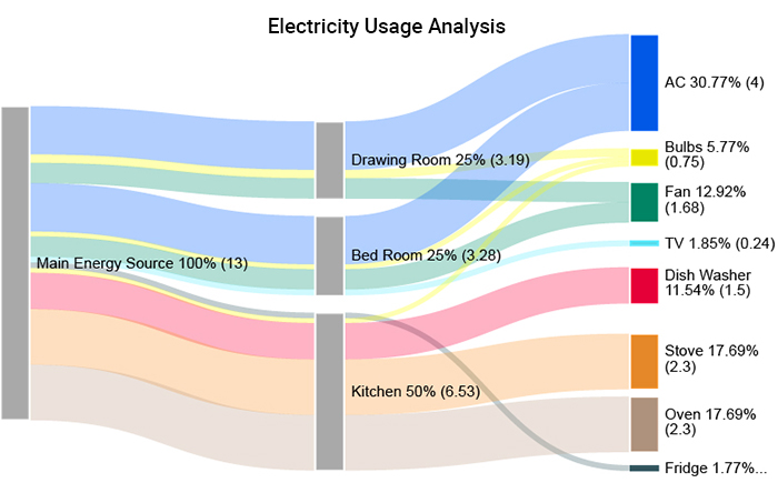
(Image source: PPCexpo, Example #2)
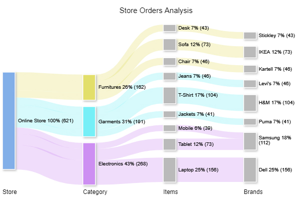
Example 2: The figure below (Figure 2) shows the classification of orders on a shopping website: starting from total orders, broken down by product category, subcategory, and brand; link width represents order quantity, and colors distinguish product categories.
We previously used plotly.express — Plotly’s high-level interface for creating common charts with simple functions. Drawing Sankey diagrams requires the lower-level interface plotly.graph_objects.
Low-Level Interface: Provides basic functions that directly manipulate underlying data, requiring more code to write.
High-Level Interface: Provides highly integrated functions that are convenient to use but less flexible.
For example,matplotlib.pyplotis Matplotlib’s high-level interface (plt.hist()), while importing the lower-levelmatplotlibmodule gives access to functions likempl.axes.Axes().
# Import plotly via low-level interface, aliased as go
import plotly.graph_objects as goWe will use go.Sankey() to store Sankey diagram data, then use go.Figure() to render it. Strictly speaking, go.Sankey() is a constructor of a class, and calling it creates an object that stores the Sankey diagram data; the same applies to go.Figure().
Common Python terminology relationships are shown in Table 1:
pd, go are library interfaces; df is a concrete object)
| Concept | Related Concept | Example |
|---|---|---|
| Function | Parameter | pd.read_csv( |
| Object | Method | df.sample(size=10) |
| Class | Property | go.Sankey(node=..., link=...) |
| Object | Attribute | df.columns |
A dictionary (dict) is a Python data structure that stores data as key-value pairs. There are three common ways to create one:
# Method 1
d1 = {'a': 1, 'b': 2, 'c': 3}  # keys must be quoted

# Method 2
d2 = dict(a=1, b=2, c=3)  # no quotes needed

# Method 3
keys = ['a', 'b', 'c']  # define keys and values separately
values = [1, 2, 3]
d3 = dict(zip(keys, values))  # zip() pairs them together, dict() converts to a dictionary

print(d1)
print(d2)
print(d3)
{'a': 1, 'b': 2, 'c': 3}
{'a': 1, 'b': 2, 'c': 3}
{'a': 1, 'b': 2, 'c': 3}Key differences between lists and dictionaries:
# Example: animals and their sounds
animal_with_sound = {'cat': 'meow', 'dog': 'woof', 'duck': 'quack'}
sound = ['meow', 'woof', 'quack']
# List: access elements by position (index)
sound[0]'meow'# Dict: access values by key (note: dicts are unordered, cannot use index)
animal_with_sound['cat']'meow'References:
Plotly Official Sankey Diagram Tutorial
plotly.graph_objects.Sankey() Documentation
Step 1: Use go.Sankey() to create the Sankey diagram object. In the node names, A/B/C represent three stages, and numbers represent different nodes within the same stage.
# Parameter configuration for go.Sankey()

sankey_data = go.Sankey(   # define the sankey_data variable

    ##########################################################################
    # Node
    node = dict(

        # Node labels
        label = ['A1','A2','B1','B2','C1','C2'],

        # Node colors: one-to-one correspondence with node labels
        color = [
            'yellow', 'yellow', 'tomato', 'tomato',
            'cornflowerblue', 'cornflowerblue',
        ],

        # Node spacing (padding) and thickness (unit: px)
        pad = 30,
        thickness = 20,

        # Node border
        line = dict(
            color = 'black', # border color
            width = 5,       # border width (unit: px)
        )
    ),

    ##########################################################################
    # Link
    link = dict(

        # Source nodes: index in the node label list
        source = [0, 1, 0, 2, 3, 3],

        # Target nodes: index in the node label list
        target = [2, 3, 3, 4, 4, 5],

        # Link flow values: corresponding to source and target lists
        value = [8, 4, 2, 8, 4, 2],

        # Link colors: corresponding to the above
        color = [
            'sandybrown', 'sandybrown', 'sandybrown',
            'thistle', 'thistle', 'thistle',
        ],

        # Link arrow length: pointing from source to target (default 0, no arrow)
        arrowlen = 15
    )
)

##############################################################################
# Check the data type of sankey_data
print('Data type:\n', type(sankey_data),'\n')

# Check the content of sankey_data
print('Content:\n', sankey_data)
Data type:
<class 'plotly.graph_objs._sankey.Sankey'>
Content:
Sankey({
'link': {'arrowlen': 15,
'color': [sandybrown, sandybrown, sandybrown, thistle, thistle,
thistle],
'source': [0, 1, 0, 2, 3, 3],
'target': [2, 3, 3, 4, 4, 5],
'value': [8, 4, 2, 8, 4, 2]},
'node': {'color': [yellow, yellow, tomato, tomato, cornflowerblue,
cornflowerblue],
'label': [A1, A2, B1, B2, C1, C2],
'line': {'color': 'black', 'width': 5},
'pad': 30,
'thickness': 20}
})As seen from the output, sankey_data is a Plotly Sankey object, with parameters stored in nested dictionaries.
When building a Sankey object, note that values in the source and target node lists are indices into the node label list, not node names themselves. For example, 0 in source = [0, 1, 0, 2, 3, 3] refers to the first node ‘A1’, 1 refers to the second node ‘A2’, and so on. Therefore, you must ensure that indices match the order of nodes in the label list, otherwise links will point to the wrong nodes.
Step 2: Use go.Figure() to render the figure:
# Render figure
fig = go.Figure(sankey_data)

# Update layout
fig.update_layout(
    height=400,
    title_text='Sample Sankey Diagram',
    title_x=0.5, title_y=0.95, # title position
    margin=dict(
        l=60, r=60, t=60, b=20,
    ),
    font={'style': 'italic'},
)

# Display figure
# fig.show(renderer='notebook')  # if use VS Code or Jupyter, use this line
fig.show()As shown in Figure 3, A/B/C represent three stages, and numbers represent different nodes within the same stage. Link width represents flow quantity, and colors distinguish different stages or categories.
As the number of nodes grows, managing indices becomes difficult. To address this, we can define a dictionary to look up the index of a node by its name, making the data construction more intuitive:
# Define a list variable to store node names
node_names = ['A1', 'A2', 'B1', 'B2', 'C1', 'C2']

# Generate index list corresponding to nodes using range(len())
node_ids = range(len(node_names))

# Build a name-to-index dictionary
nodes = dict(zip(node_names, node_ids))nodes['B2'] # look up the index for a node by name3This allows you to look up the index of source nodes and target nodes in the node label list by name.
At the same time, for long parameters, you can pre-define variables and pass them into the function, making the code cleaner and easier to maintain. The following code redraws the same Sankey diagram shown in Figure 3 above:
##############################################################################
# Values needed for node parameters

# Define node colors
node_colors = [
    'yellow', 'yellow', 'tomato', 'tomato',
    'cornflowerblue', 'cornflowerblue',
]

# Define the complete node parameter
node_definition = dict(
    pad=15,
    thickness=20,
    line=dict(color='black', width=5),
    label=node_names,   # use the node name variable defined above
    color=node_colors,  # use the node color variable just defined
)

##############################################################################
# Values needed for link parameters

# Look up indices by node name to define sources and targets
sources = [
    nodes['A1'], nodes['A1'], nodes['A2'],
    nodes['B1'], nodes['B2'], nodes['B2'],
]
targets = [
    nodes['B1'], nodes['B2'], nodes['B2'],
    nodes['C1'], nodes['C1'], nodes['C2'],
]

# Define link flow values and colors
values = [8, 4, 2, 8, 4, 2]
link_colors = [
    'sandybrown', 'sandybrown', 'sandybrown',
    'thistle', 'thistle', 'thistle',
]

# Define the complete link parameter
link_definition = dict(
    source=sources,
    target=targets,
    value=values,
    color=link_colors,
    arrowlen=15,
)

##############################################################################
# Draw the Sankey diagram

# Pass the pre-defined node_definition and link_definition into the function
fig = go.Figure(
    go.Sankey(
        node = node_definition,
        link = link_definition,
    )
)

# Update layout
fig.update_layout(
    height=400,
    title_text='Sample Sankey Diagram - Redrawn',
    title_x=0.5, title_y=0.95,
    margin=dict(
        l=60, r=60, t=60, b=20,
    ),
    font={'style': 'italic'},
)
fig.show() # display the chartThe redrawn result is identical to the original. But by pre-defining data as variables, you only need to adjust variable values when modifying data, making the code cleaner and easier to maintain.
To modify link color transparency, use RGBA values instead of color name strings. The RGBA format is (red, green, blue, alpha), where alpha represents opacity (0 = fully transparent, 1 = fully opaque). Both "sandybrown" and "thistle" are CSS preset color names, which can be found at w3schools CSS Colors or the Matplotlib Color Reference.
# Import library for handling RGBA values
import matplotlib.colors as c
# Use c.to_rgba() to find RGB values and set alpha
c.to_rgba('sandybrown', 0.5)(0.9568627450980393, 0.6431372549019608, 0.3764705882352941, 0.5)Plotly supports specifying RGBA colors using the string format 'rgba(r, g, b, a)'.
# Define strings to store RGBA values for transparent colors
faint_sandybrown = 'rgba' + str(c.to_rgba('sandybrown', 0.5)) # + concatenates strings
faint_thistle = 'rgba' + str(c.to_rgba('thistle', 0.5))

# Print the strings
print(faint_sandybrown)
print(faint_thistle)
rgba(0.9568627450980393, 0.6431372549019608, 0.3764705882352941, 0.5)
rgba(0.8470588235294118, 0.7490196078431373, 0.8470588235294118, 0.5)# Redefine link colors
link_colors = [
faint_sandybrown, faint_sandybrown, faint_sandybrown,
faint_thistle, faint_thistle, faint_thistle,
]
# Update chart
fig.update_traces(link_color=link_colors)
fig.update_layout(
height=400,
title_text='Sample Sankey Diagram - 50% Link Transparency',
title_x=0.5, title_y=0.95,
margin=dict(
l=60, r=60, t=60, b=20,
),
font={'style': 'italic'},
)
fig.show()Both Sankey diagrams and network graphs visualize relational data, but with different emphases, as shown in Table 2:
| Feature | Sankey Diagram | Network Graph |
|---|---|---|
| Primary Use | Visualize resource flow quantities | Visualize connections between nodes |
| Node Meaning | Process stage or entity | Individual (e.g., a user) |
| Connection Name | Link | Edge |
| Connection Direction | Directed (source → target) | Can be directed or undirected |
| Connection Width | Represents flow quantity | No width distinction |
| Key Characteristics | Hierarchical, flow conservation | Connection strength and relational distance |
| Application Examples | Energy distribution, cost allocation | Social networks, computer networks |
Install pyvis before use (includes networkx).
pip install pyvisIn a local environment (Jupyter), installation persists and can be reused; in Google Colab’s virtual environment, installation only applies to the current file and must be repeated for new files.
# Import libraries for drawing network graphs
from pyvis.network import Network
import networkx as nx
Step 1: Create network relationships with networkx
# Create an empty undirected graph
gx = nx.Graph()
# Note: use nx.MultiDiGraph() to create a directed graph instead
# Add nodes and edges to the empty graph gx
gx.add_edge('a', 'b') # edge from 'a' to 'b'
gx.add_edge('b', 'd')
gx.add_edge('c', 'e')
gx.add_edge('e', 'a')
gx.add_edge('c', 'd')Step 2: Output an interactive network graph with pyvis
# Create an empty interactive network graph object
gp = Network()

# Load network relationships from gx
gp.from_nx(gx)

# Output as a standalone HTML file
gp.show('net.html', notebook=False)
# notebook=False let the fig not be rendered in Jupyter output cell
# only use True when you are using Jupyter & browser
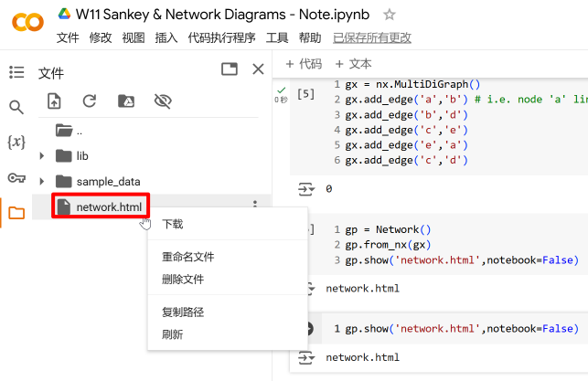
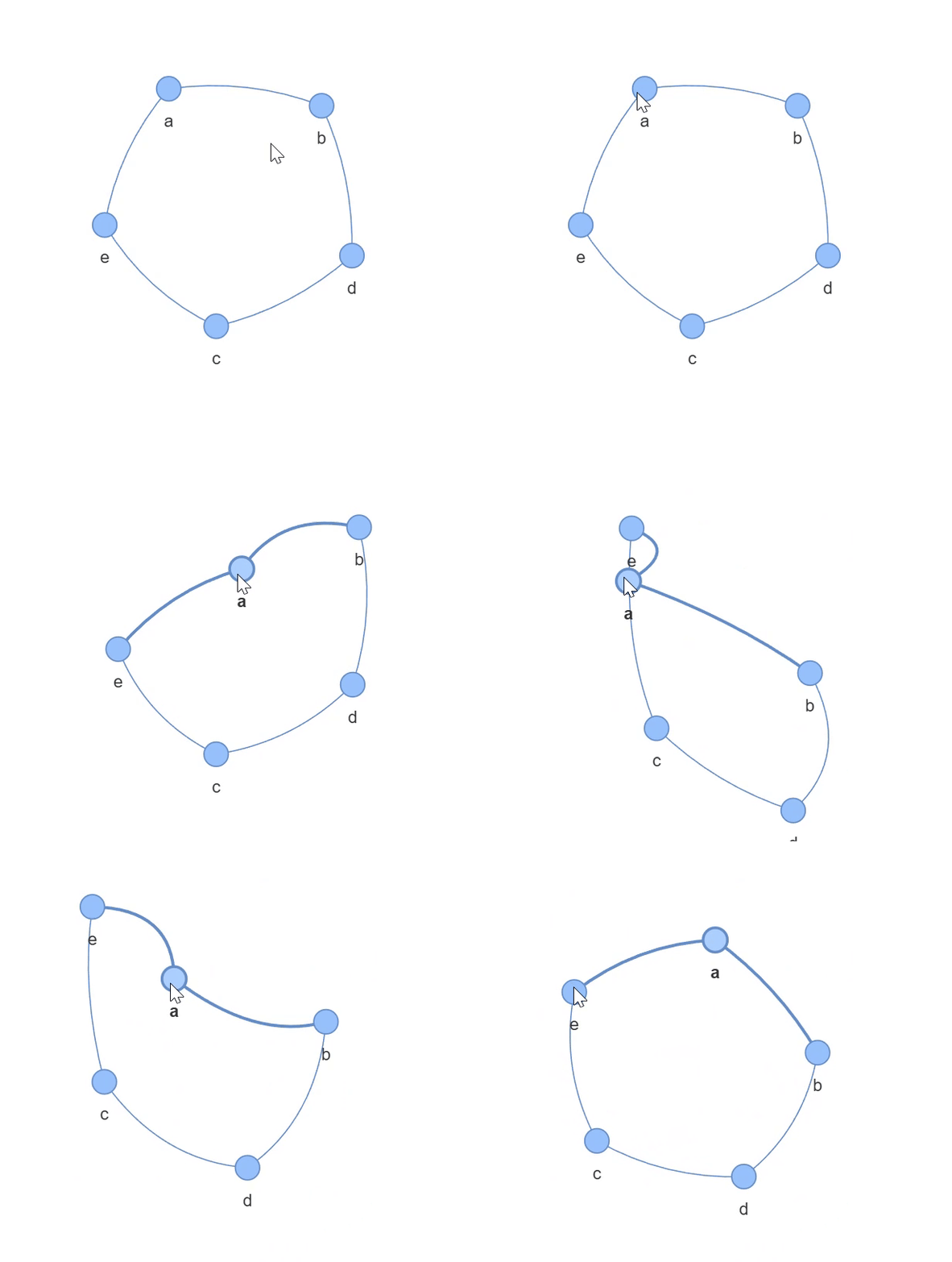
The output standalone HTML file is saved in the current directory (view source code and files). In Colab, it can be found in the left file panel, as shown in Figure 6. Download it and open it in a browser to see the result shown in Figure 7.
print(gp.nodes[0]) # view info for the first node (index 0){'color': '#97c2fc', 'size': 10, 'id': 'a', 'label': 'a', 'shape': 'dot'}Manually modifying node attributes:
# Modify node attributes
gp.nodes[0]['color'] = 'red' # color
gp.nodes[0]['size'] = 20     # size

# Rename the output file to avoid overwriting the original
gp.show('net-modified.html', notebook=False)
The modified result is shown in Figure 8:
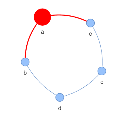
There are a few approaches to render interactive network diagrams in output cells (see this blog). Below shows the approach with the most adaptability that can render networks in any environment without external files or dependencies.
from IPython.display import HTML, display

# store network's html code
html = gp.generate_html()

# format: only use double quotes
html_formatted = html.replace("'",'"')

# defining iframe tag
iframe_start = """
<iframe
sandbox='allow-scripts allow-forms'
style='display:block; margin:0px; width:100%; aspect-ratio:3/2;'
frameborder='0'
srcdoc='
"""
iframe_end = " '></iframe> "

# wrap formatted html code with iframe tag
html_wrapped = iframe_start + html_formatted + iframe_end

# display
display(HTML(html_wrapped))In addition to manual creation, network relationship data can also be read from a CSV file. The following example uses beer and curry tweet data (view source file): original posters mentioned other users, forming directed edges from the original poster (source node) to the mentioned user (target node).
###############################################################################
# Data preprocessing

# Import pandas to handle the CSV file
import pandas as pd

# Read the CSV file
path = '../../../src/data/beer-and-curry.csv'
df = pd.read_csv(path)

# Drop rows with no mentions
df.dropna(subset='mentions', inplace=True)

###############################################################################
# Create network relationships

# Create an empty directed graph
gx1 = nx.MultiDiGraph()

# Loop over all rows
for i in df.index:
    user = df.loc[i, 'user']              # get the user as source node
    mentions = df.loc[i, 'mentions']      # get all mentions in a post
    mentions = mentions.replace(' ', '')  # remove spaces
    mentions = mentions.split('@')        # split by '@' to get individual mentions
    mentions.pop(0)                       # first element after split is empty, remove it

    for mention in mentions:
        gx1.add_edge(user, mention)       # add all nodes and edges

###############################################################################
# Draw the network graph

gp1 = Network()   # create an empty network graph
gp1.from_nx(gx1)  # load network relationships
gp1.show('net-from-csv.html', notebook=False)  # output HTML file
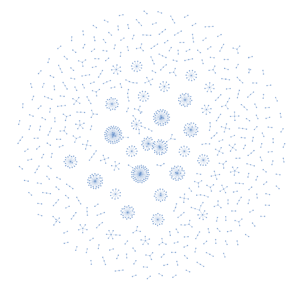
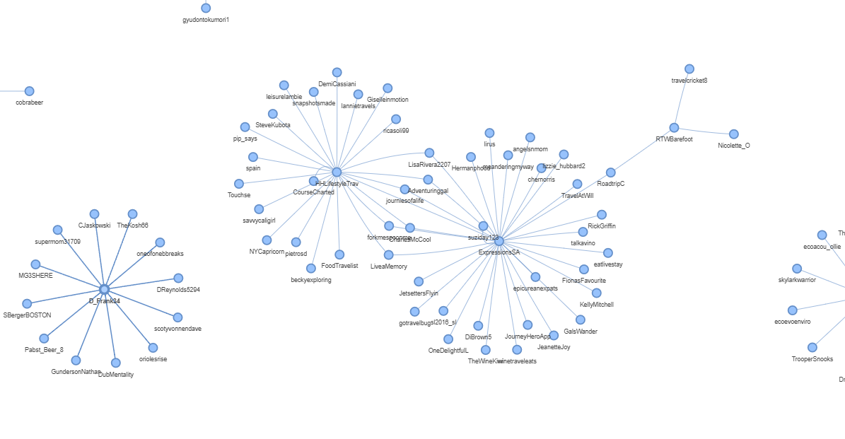
The output network graph is complex; rendering may take 1–2 minutes — do not close the browser during this time. The overall view is shown in Figure 9, and a detail view in Figure 10.
Network graphs can be used to study social networks, identify strong/weak connections and high-influence users, and analyze potential information cocoon or echo chamber phenomena.