Data Processing

Data processing/cleaning workflows in Pandas: missing values, duplicates, reshaping, joins, aggregations, pivoting, etc.

9 min read · 1708 EN words · 0 中文字

python==3.12
pandas==2.2.2

1 Handling Missing Values

Reading CSV Files:

• Use pd.read_csv(path) to load a CSV file into a Pandas DataFrame.
  
• Ensure path separators use forward slashes / (or escaped backslashes \\ for Win).

# import data
import pandas as pd
path = "../../../src/data/beer-and-curry.csv"
df = pd.read_csv(path) # read csv file into a DataFrame
df.head(2) # view first 2 rows

	created_at	utc_time	mentions	text	url	retweet_count	favorite_count	user	user.location	user.followers_count	user.friends_count	user.created_at	user.favourites_count	user.verified
0	06/05/2020	11:11:49	NaN	NINE SPICES?????????????????\n?9??SPICE????NIN...	https://t.co/wddjIaJTcD	24	12	9spices	??????????2-1-2 HANROKU??B1	3820	1961	10/02/2010	296	False
1	07/07/2020	08:08:54	@lizzie_hubbard2 @JetsettersFlyin @suziday123 ...	Thanks for the invite to join #TravelWinePart...	https://t.co/6Z7GgkJE8v	6	17	ExpressionsSA	Cape Town South Africa	5088	5284	24/06/2011	15625	False

1.1 Dropping Missing Values

Use dropna() to remove rows with missing values in the columns required for analysis.

# drop rows where 'text' or 'retweet_count' is missing (value is NA or NaN)
df_clean = df.dropna(subset=["text", "retweet_count"])

Dropping Missing Values:

• Use df.dropna() to remove rows containing missing values (NA or NaN).
  
• By default, it removes any row with at least one missing value.
  
• Specify subset as a list of column names to only consider missing values in those columns for removal.
  
• Use parentheses () or square brackets [] for the subset list.

Note: For data preprocessing, selectively drop rows with missing values only in columns relevant to your analysis to maintain data accuracy.

df.shape # view original shape (num of rows, num of cols)

(430, 14)

df_clean.shape # shape after dropping rows with missing values

(429, 14)

1.2 Filling Missing Values

Use fillna() when a missing value should be replaced rather than removed.

# fill missing values in 'mentions' with a placeholder string
df["mentions"] = df["mentions"].fillna("No Mentioned User")

# view replaced values in 'mentions' column
df.head(3)["mentions"]

0                                    No Mentioned User
1    @lizzie_hubbard2 @JetsettersFlyin @suziday123 ...
2    @craftbeerncl! @RidgesideBrewer @Manjitskitche...
Name: mentions, dtype: object

Filling Missing Values:

• Use df.fillna(value) to replace missing values in a specific column with a placeholder, such as a string.
  
• Assign the result back to the column to update the DataFrame.

1.3 Replacing Specific Values

Use replace() to convert placeholder values into a more useful representation.

# replace the placeholder string with 0
df["mentions"] = df["mentions"].replace("No Mentioned User", 0)

# view replaced values in 'mentions' column
df.head(3)["mentions"]

0                                                    0
1    @lizzie_hubbard2 @JetsettersFlyin @suziday123 ...
2    @craftbeerncl! @RidgesideBrewer @Manjitskitche...
Name: mentions, dtype: object

Replacing Specific Values:

• Use df.replace(old_value, new_value) to substitute specific values in a column.
  
• This is useful for converting placeholders into more appropriate representations, like numbers.

2 Renaming and Creating Columns

2.1 Renaming Columns

Use rename() to make column names shorter and more descriptive.

# rename 'text' to 'content' and 'created_at' to 'date'
df = df.rename(columns={"text": "content", "created_at": "date"})

# view renamed columns
df.head(2)

	date	utc_time	mentions	content	url	retweet_count	favorite_count	user	user.location	user.followers_count	user.friends_count	user.created_at	user.favourites_count	user.verified
0	06/05/2020	11:11:49	0	NINE SPICES?????????????????\n?9??SPICE????NIN...	https://t.co/wddjIaJTcD	24	12	9spices	??????????2-1-2 HANROKU??B1	3820	1961	10/02/2010	296	False
1	07/07/2020	08:08:54	@lizzie_hubbard2 @JetsettersFlyin @suziday123 ...	Thanks for the invite to join #TravelWinePart...	https://t.co/6Z7GgkJE8v	6	17	ExpressionsSA	Cape Town South Africa	5088	5284	24/06/2011	15625	False

Renaming Columns:

• Use df.rename(columns={'old_name': 'new_name'}) to rename columns using a dictionary.
  
• This improves readability and descriptiveness.
  
• Similarly, use index parameter for renaming indices.

2.2 Creating New Columns

Drop rows with missing follower counts before creating derived metrics.

# specify specific column(s) to drop rows with missing values
df = df.dropna(subset=["user.followers_count"])

# view cleaned data with no missing follower counts
df.head(2)

	date	utc_time	mentions	content	url	retweet_count	favorite_count	user	user.location	user.followers_count	user.friends_count	user.created_at	user.favourites_count	user.verified
0	06/05/2020	11:11:49	0	NINE SPICES?????????????????\n?9??SPICE????NIN...	https://t.co/wddjIaJTcD	24	12	9spices	??????????2-1-2 HANROKU??B1	3820	1961	10/02/2010	296	False
1	07/07/2020	08:08:54	@lizzie_hubbard2 @JetsettersFlyin @suziday123 ...	Thanks for the invite to join #TravelWinePart...	https://t.co/6Z7GgkJE8v	6	17	ExpressionsSA	Cape Town South Africa	5088	5284	24/06/2011	15625	False

Creating New Columns:

• First, clean the data by dropping rows with missing values in relevant columns using df.dropna(subset=['column']).

2.2.1 Applying Basic Column Operations

Create a new column by applying a vectorized calculation to an existing column.

# create a new column 'followers_k' by dividing 'user.followers_count' by 1000
df["followers_k"] = df["user.followers_count"] / 1000

# view the new column alongside the original follower count
df.head(3)[["followers_k", "user.followers_count"]]

	followers_k	user.followers_count
0	3.820	3820
1	5.088	5088
2	0.446	446

Creating New Columns:

• Create new columns by performing vectorized operations on existing columns, e.g., df['new_col'] = df['existing_col'] / 1000.

2.2.2 Applying a Custom Function

Define a reusable function when the transformation is clearer as named logic.

# define a function to calculate engagement rate (ER) as a percentage
def calc_er(engagement_count, follower_count):
    return (engagement_count / follower_count) * 100

# apply and assign the calculated engagement rate to a new column 'er_rt_fo'
df["er_rt_fo"] = calc_er(
    df["retweet_count"],
    df["user.followers_count"],
)

# view the new engagement rate column alongside the original metrics
df.head(3)[["er_rt_fo", "retweet_count", "user.followers_count"]]

	er_rt_fo	retweet_count	user.followers_count
0	0.628272	24	3820
1	0.117925	6	5088
2	0.896861	4	446

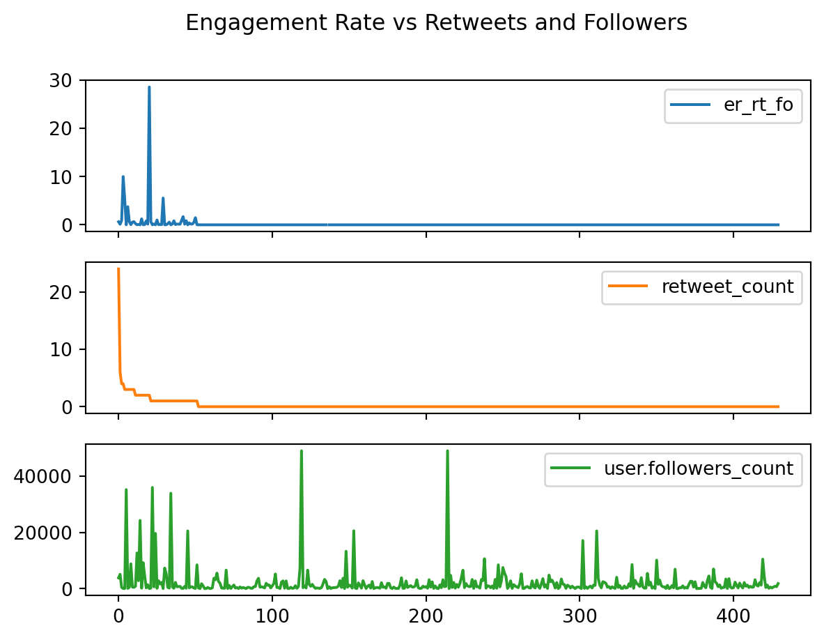
# visualize the relationship between engagement rate & two other metrics
ax = df[["er_rt_fo", "retweet_count", "user.followers_count"]].plot(
    subplots=True,
    title="Engagement Rate vs Retweets and Followers",
)

Creating New Columns:

• Define a function for complex calculations, such as efficiency ratio: ER = (effective cost / full cost) * 100.
  
• Apply the function to DataFrame columns to generate new metrics.
  
• Use .values if needed to extract array from Series.
  
• Visualize relationships using df.plot() with subplots=True for separate plots, figsize for dimensions, and kind for plot types (default ‘line’, options include ‘bar’, ‘hist’, ‘scatter’, ‘pie’).

3 Finding Duplicates

Remove fully duplicated rows with duplicated().

# drop fully duplicated rows (keep the first occurrence)
# ~ is the negation operator
df = df[~df.duplicated()]

Finding Duplicates:

• Use df.duplicated() to identify duplicate rows; it returns a boolean Series.
  
• Use ~df.duplicated() to keep only unique rows.
  
• Specify subset as a list of columns to check for duplicates based on those columns only.
  
• Use keep=False to mark all duplicates.

Find users who posted multiple times on the same date by specifying a subset of columns.

# find duplicated rows based on 'user' and 'date' columns (keep all occurrences)
df[df.duplicated(subset=["user", "date"], keep=False)].head(2)

	date	utc_time	mentions	content	url	retweet_count	favorite_count	user	user.location	user.followers_count	user.friends_count	user.created_at	user.favourites_count	user.verified	followers_k	er_rt_fo
7	29/02/2020	14:42:01	@MCRCycleSam @CatrionaSwanson @bricycle @marty...	A gathering of UK transport activists; cycle s...	https://t.co/OcyyKkhmUh	3	15	davelostdave	somewhere	459	1287	15/06/2009	23700	False	0.459	0.653595
10	29/02/2020	23:41:58	@CatrionaSwanson @Chris_Boardman @Chris_Boardman	Maybe we could put the spotlight on #Bradford ...	https://t.co/0ExO7wr1ld	3	11	davelostdave	somewhere	459	1287	15/06/2009	23700	False	0.459	0.653595

4 Reordering and Reshaping Data

Sort rows by multiple columns with sort_values().

# sort by 'retweet_count' and then by 'user.followers_count' descending
df.sort_values(
    by=["retweet_count", "user.followers_count"],
    ascending=False,
).head(2)

	date	utc_time	mentions	content	url	retweet_count	favorite_count	user	user.location	user.followers_count	user.friends_count	user.created_at	user.favourites_count	user.verified	followers_k	er_rt_fo
0	06/05/2020	11:11:49	0	NINE SPICES?????????????????\n?9??SPICE????NIN...	https://t.co/wddjIaJTcD	24	12	9spices	??????????2-1-2 HANROKU??B1	3820	1961	10/02/2010	296	False	3.820	0.628272
1	07/07/2020	08:08:54	@lizzie_hubbard2 @JetsettersFlyin @suziday123 ...	Thanks for the invite to join #TravelWinePart...	https://t.co/6Z7GgkJE8v	6	17	ExpressionsSA	Cape Town South Africa	5088	5284	24/06/2011	15625	False	5.088	0.117925

Reordering and Reshaping:

• Use df.sort_values(by=['col1', 'col2'], ascending=False) to sort rows by multiple columns in descending order.
  
• Use df.transpose() to swap rows and columns.

Transpose the DataFrame when you need to switch rows and columns for inspection.

df.transpose().head(3) # view the DataFrame with rows and columns swapped

	0	1	2	3	4	5	6	7	8	9	...	420	421	422	423	424	425	426	427	428	429
date	06/05/2020	07/07/2020	31/03/2020	29/05/2020	28/11/2020	01/07/2020	08/01/2020	29/02/2020	03/05/2020	16/01/2020	...	10/04/2020	27/11/2020	09/12/2020	25/03/2020	25/06/2020	30/12/2020	30/08/2020	04/03/2020	10/08/2020	07/03/2020
utc_time	11:11:49	08:08:54	13:39:02	20:58:17	04:46:37	06:35:04	10:26:36	14:42:01	17:05:51	17:50:08	...	23:23:26	23:31:09	23:32:06	23:36:02	23:38:41	23:45:00	23:54:19	23:55:19	23:55:38	23:59:42
mentions	0	@lizzie_hubbard2 @JetsettersFlyin @suziday123 ...	@craftbeerncl! @RidgesideBrewer @Manjitskitche...	@StCannas @keralankaravan	@yooneedmorejodi	0	0	@MCRCycleSam @CatrionaSwanson @bricycle @marty...	@DrewPritchard	@Nellachops73 @MotorheadBeer @CameronsBrewery ...	...	@ashley_collings	@101andyhibberd	@MariaMo71609443 @jckiker @ScottAdamsSays	@lonelyplanet	0	@Photos_in_Chile	@jesshousty @WilliamHousty	@beer_porter @siretoknote	0	0

3 rows × 430 columns

5 Joining Data

Load a second dataset and combine it with concat().

path2 = "../../../src/data/keto-and-vegan.csv"
df2 = pd.read_csv(path2, encoding="latin-1") # load df
df2.head(2) # view first 2 rows

	created_at	utc_time	mentions	text	url	retweet_count	favorite_count	user	user.location	user.followers_count	user.friends_count	user.created_at	user.favourites_count	user.verified
0	01/01/2020	23:10:27	@BioLayne	is one of the most respected and unbiased nutr...	https://t.co/WDDhoIvXl5	0	0	Eric_OGrey	Sacramento, CA	2333	1084	10/03/2016	23996	False
1	02/01/2020	18:16:26	@greggprescott1	I am O +, which is high protein, than fat, the...	https://t.co/1hBpp6MGnu	0	0	Glory32X	Belgium	636	64	11/07/2009	22357	False

Append matching tables vertically:

# concatenate df and df2 vertically (stack rows)
pd.concat([df, df2]).iloc[428:432,] # view row 428 to 431

	date	utc_time	mentions	content	url	retweet_count	favorite_count	user	user.location	user.followers_count	user.friends_count	user.created_at	user.favourites_count	user.verified	followers_k	er_rt_fo	created_at	text
428	10/08/2020	23:55:38	0	Made the terrible horrible no-good mistake of ...	https://t.co/AF23qFRBTv	0	3	elizvogt	NYC now, Texas forever	687	1105	07/03/2011	39909	False	0.687	0.0	NaN	NaN
429	07/03/2020	23:59:42	0	This is how I'm celebrating tonight y'all! Bee...	https://t.co/Fh7wRYCguR	0	30	Rose262	Atlanta, GA	1776	1121	10/05/2009	30246	False	1.776	0.0	NaN	NaN
0	NaN	23:10:27	@BioLayne	NaN	https://t.co/WDDhoIvXl5	0	0	Eric_OGrey	Sacramento, CA	2333	1084	10/03/2016	23996	False	NaN	NaN	01/01/2020	is one of the most respected and unbiased nutr...
1	NaN	18:16:26	@greggprescott1	NaN	https://t.co/1hBpp6MGnu	0	0	Glory32X	Belgium	636	64	11/07/2009	22357	False	NaN	NaN	02/01/2020	I am O +, which is high protein, than fat, the...

Joining Data:

• Load additional datasets with pd.read_csv() and specify encoding if necessary.
  
• Use pd.concat([df1, df2]) to vertically concatenate DataFrames with matching columns.
  
• Reset the index with .reset_index(drop=True) to create a continuous index.

Reset the index after concatenation when you want a continuous row index.

# concatenate df and df2, then reset the index
pd.concat([df, df2]).reset_index(drop=True).iloc[428:432,]

	date	utc_time	mentions	content	url	retweet_count	favorite_count	user	user.location	user.followers_count	user.friends_count	user.created_at	user.favourites_count	user.verified	followers_k	er_rt_fo	created_at	text
428	10/08/2020	23:55:38	0	Made the terrible horrible no-good mistake of ...	https://t.co/AF23qFRBTv	0	3	elizvogt	NYC now, Texas forever	687	1105	07/03/2011	39909	False	0.687	0.0	NaN	NaN
429	07/03/2020	23:59:42	0	This is how I'm celebrating tonight y'all! Bee...	https://t.co/Fh7wRYCguR	0	30	Rose262	Atlanta, GA	1776	1121	10/05/2009	30246	False	1.776	0.0	NaN	NaN
430	NaN	23:10:27	@BioLayne	NaN	https://t.co/WDDhoIvXl5	0	0	Eric_OGrey	Sacramento, CA	2333	1084	10/03/2016	23996	False	NaN	NaN	01/01/2020	is one of the most respected and unbiased nutr...
431	NaN	18:16:26	@greggprescott1	NaN	https://t.co/1hBpp6MGnu	0	0	Glory32X	Belgium	636	64	11/07/2009	22357	False	NaN	NaN	02/01/2020	I am O +, which is high protein, than fat, the...

6 Grouping and Aggregation

Use groupby() with agg() to compute summary statistics by group. The example below calculates total retweets and average follower count for each user.

# group by 'user', then aggregate 'retweet_count' with sum 
# and 'user.followers_count' with mean
df_agg = df.groupby("user").agg(
    {"retweet_count": "sum", "user.followers_count": "mean",}
)

# view the aggregated result
df_agg.head(3)

	retweet_count	user.followers_count
user
1nnkeeper	0	557.0
353a9f40f97e4a9	2	4440.0
6M70_JET	0	548.0

Grouping and Aggregation:

• Use df.groupby('column').agg({'col1': 'sum', 'col2': 'mean'}) to group by a column and compute aggregate statistics.
  
• Verify the number of groups using df[~df.duplicated(subset='column')].shape or df['column'].nunique().

You can compare the grouped result with the number of unique users:

# count unique users by dropping duplicates based on 'user' column
df[~df.duplicated(subset="user")].shape

(390, 16)

# or simply count the number of unique users with nunique()
df["user"].nunique()

390

7 Melting and Pivoting

7.1 Melting Data

Melting: wide → long

Use melt() to convert wide data into long format for analysis and plotting.

# create a sample wide-format DataFrame with pet types and counts
df_wide = pd.DataFrame(
    data=[
        ["cat", 4, 5],
        ["dog", 7, 4],
        ["rabbit", 2, 3],
    ],
    columns=["pet", "male", "female"],
)

df_wide # view it

	pet	male	female
0	cat	4	5
1	dog	7	4
2	rabbit	2	3

Without arguments, melt() collapses all columns into variable-value pairs.

df_wide.melt() # melt all cols into variable-value pairs (pivot longer)

	variable	value
0	pet	cat
1	pet	dog
2	pet	rabbit
3	male	4
4	male	7
5	male	2
6	female	5
7	female	4
8	female	3

Specify identifier and value columns for a structured long-format result.

melted_df = pd.melt(
    df_wide,
    id_vars=["pet"], # keep 'pet' as identifier column
    value_vars=["male", "female"], # value columns
    var_name="sex", # name for the new variable column
    value_name="count", # name for the new value column
)

7.2 Pivoting Data

Pivot: long → wide

Pivot the long data back to wide format:

df_pivot = melted_df.pivot(
    index="pet", # identifier column becomes index
    columns="sex", # categories in variable column becomes new columns
    values="count", # value column becomes new values
).reset_index() # reset index to turn 'pet' back into a column

df_pivot.columns.name = None # remove the name of the columns index

df_pivot # view the pivoted DataFrame

	pet	female	male
0	cat	5	4
1	dog	4	7
2	rabbit	3	2

Use pivot_table() instead of pivot() when there are duplicate index/column combinations, and specify an aggregation function like aggfunc='mean' to summarize duplicates.

For example, if we have duplicate pet entries:

# create a sample DataFrame with duplicate pet entries
df_long = pd.DataFrame(
    data=[
        ["cat", "male", 4],
        ["cat", "female", 5],
        ["dog", "female", 7],
        ["dog", "male", 4],
        ["rabbit", "male", 2],
        ["rabbit", "female", 3],
    ],
    columns=["pet", "sex", "count"],
)
df_long # view the long-format DataFrame with duplicates

	pet	sex	count
0	cat	male	4
1	cat	female	5
2	dog	female	7
3	dog	male	4
4	rabbit	male	2
5	rabbit	female	3

To pivot this long data back to wide format, we can use pivot_table() to handle duplicates:

# create a pivot table that averages counts for duplicate entries
(df_long
.pivot_table(
    index="pet",
    columns="sex",
    values="count",
    aggfunc="mean", # average counts for duplicate entries
)
.rename_axis(None, axis=1) # remove the name of the columns headers
.rename_axis(None) # remove the name of the index
)

	female	male
cat	5.0	4.0
dog	7.0	4.0
rabbit	3.0	2.0