Environment and Versions
python==3.12
pandas==2.2.2
matplotlib==3.9.x
seaborn==0.13.2Pinn Xu
October 27, 2024
“Tidy/flat” tabular data: Each row is one observation (also called instance or record), and each column is one variable (also called attribute, feature, or parameter).
Typically, multivariate refers to data with more than two variables — a multivariate plot generally uses three or more columns from the original DataFrame.
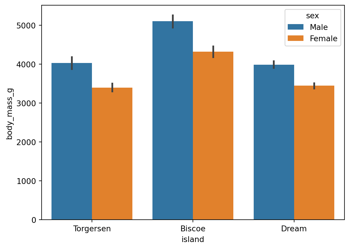
When creating a bar chart, in addition to the x and y variables, you can also set the hue parameter to include a third variable. For example, Figure 1 includes three variables: 'island', 'body_mass_g', and 'sex'.
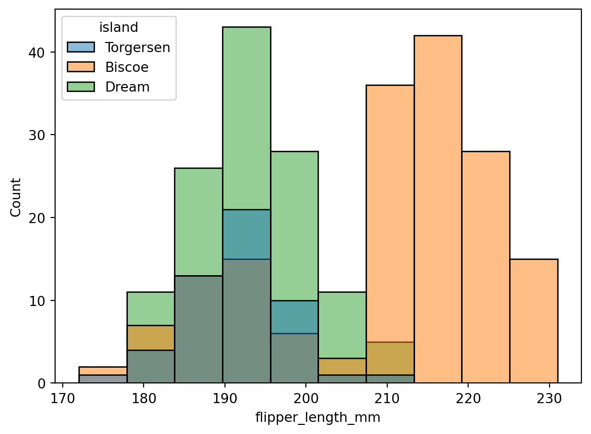
However, some chart types do not support setting x, y, and hue all at once. For example, a histogram only supports x and hue (see Figure 2): the x-axis shows distribution intervals of flipper length, and the y-axis shows the number of penguins in each interval, involving only two variables.
A facet grid (FacetGrid) is a common method for displaying multivariate data. Several small charts (facets) are arranged in a grid to form a facet grid. If you want to display a histogram while also showing more than two variables, you can use a facet grid.
The method for creating a facet grid with Seaborn is as follows:
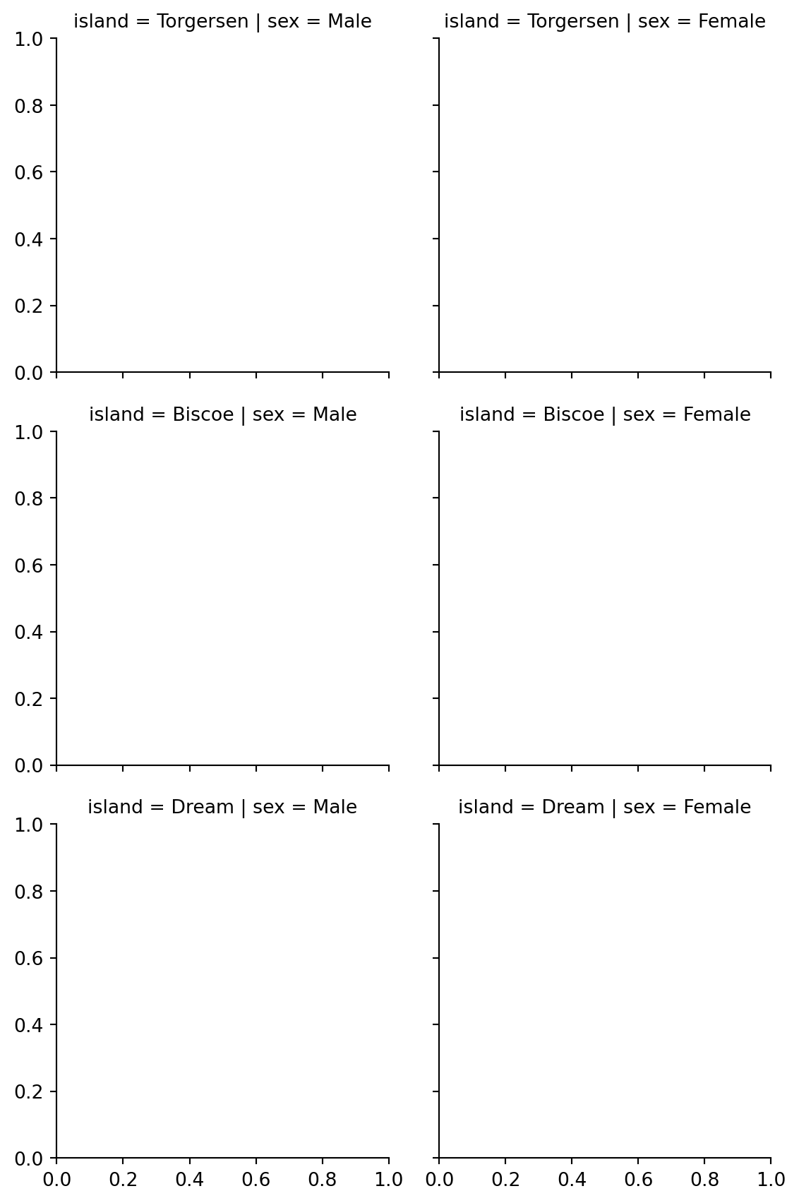
As shown in Figure 3, we created a 3×2 facet grid, but it is currently empty. Use the .map_dataframe() method to specify the content to fill in.
# fill the complete facet grid
# Step 1: create facet grid
g = sns.FacetGrid(
data=df,
col='sex',
row='island',
hue='species',
)
# Step 2: fill with histograms
g.map_dataframe(
sns.histplot,
x='flipper_length_mm',
stat='density', # sum of bar areas equals 1 for each group
common_norm=False, # each color normalized independently within each facet
)
# Step 3: add and adjust legend
g.add_legend()
sns.move_legend(
g,
loc='lower center',
bbox_to_anchor=(0.5, 1),
ncol=3, # number of legend columns
)
plt.show()stat and common_norm stat='density' uses frequency density for plotting, so the total area of all bars in the histogram sums to 1. common_norm=False is used alongside stat, meaning each color’s bars within the same facet are normalized independently, rather than all colors being normalized together.
loc and bbox_to_anchor Setting both parameters together positions the lower-center edge of the legend at coordinates (0.5, 1) of the entire grid figure. If only loc='lower center' is set, the legend will be placed at the lower center of the grid figure directly.
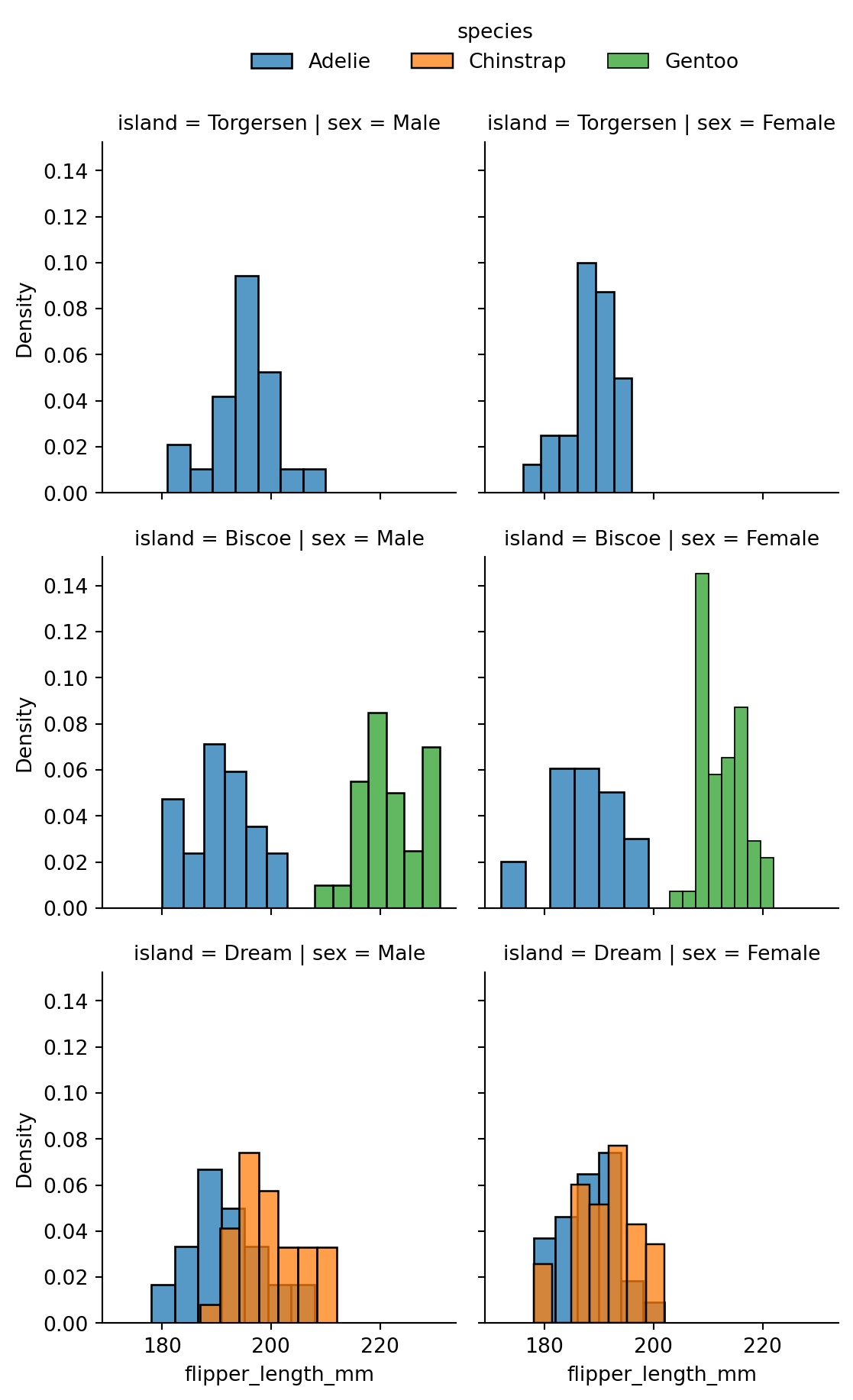
As shown in Figure 4, the facet grid separates rows by island, columns by sex, and colors by species, simultaneously displaying four variables (flipper length, island, sex, species). Splitting by rows and columns allows two additional discrete variables; color differentiation can add one more discrete variable.
Note: Because of how rows and columns work, facet grids can only add discrete variables. To facet by a continuous variable, first bin it into intervals and save as a new discrete variable column, then use the facet grid for row or column splitting.
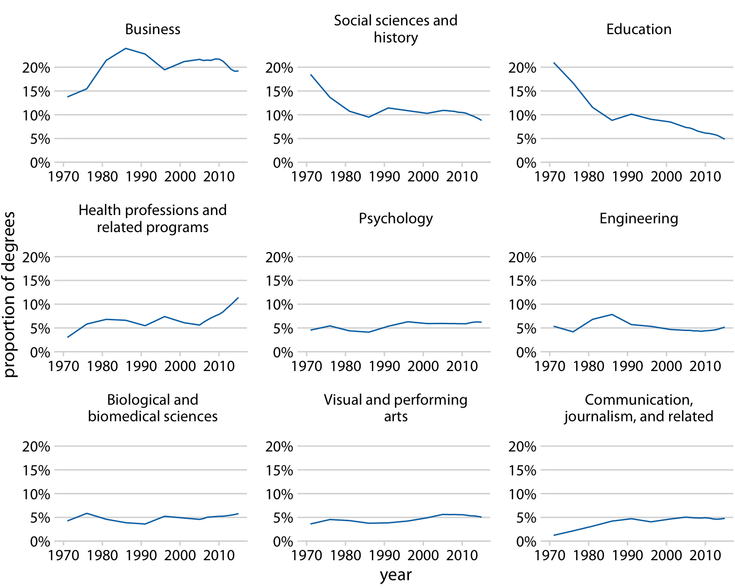
Consistent Axis Ranges When displaying multiple subplots together, each subplot should have the same axis range, because readers tend to assume that axis ranges are consistent across panels — inconsistency can lead to misinterpretation (Wilke, 2019, pp. 257-258).
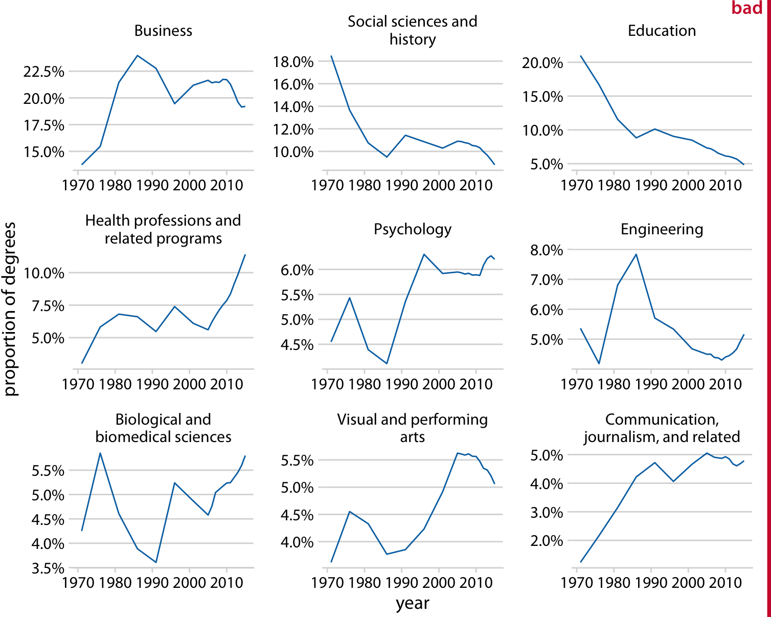
In Figure 5, each subplot has a different y-axis range, which is easy to misread. Changing to Figure 6 with consistent axis ranges across all subplots reduces reading difficulty.
Before creating scatter plots, it is important to distinguish between scatter plots and point plots.
Note: Point plots are also called dot plots (Wilke, 2019, p.43). The following distinction between scatter plots and point plots is based on the Seaborn library and may differ in other contexts.
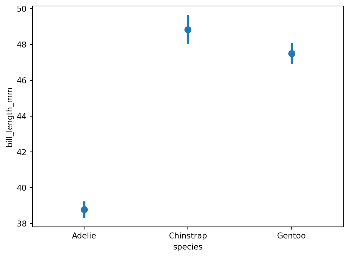
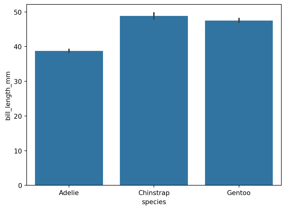
A point plot can function similarly to a bar chart: the vertical line at each point is equivalent to a bar in a bar chart, and the point corresponds to the midpoint of the top edge of each bar. Like a bar chart, a point plot can be used for category-amount charts (see Figure 7 and Figure 8):
As shown in Figure 7 and Figure 8, both point plots and bar charts can represent category-amount relationships. One key difference is that the amount axis in a bar chart must start at 0, while a point plot does not. Both point plots and bar charts only show the mean of the y-axis values (or other statistics such as the median), with each x-axis value corresponding to only one y-axis value.
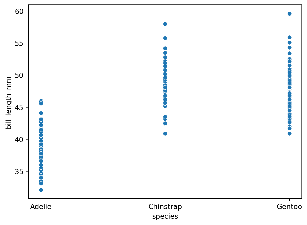
A scatter plot displays every individual data point (see Figure 9):
In a scatter plot, each x-axis value can correspond to multiple y-axis values, while in a point plot each x-axis value corresponds to only one y-axis value.
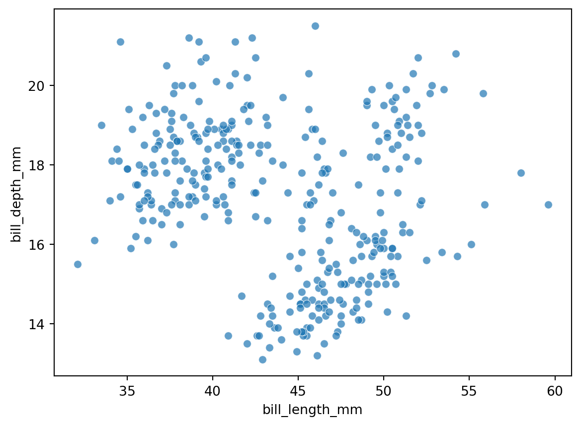
Scatter plots are commonly used to explore the relationship between two (or more) variables and to examine whether correlations exist, primarily between two continuous numeric variables. The x-axis of a scatter plot is therefore usually ratio data, with tick marks automatically displayed as a continuous numeric range (see Figure 10):
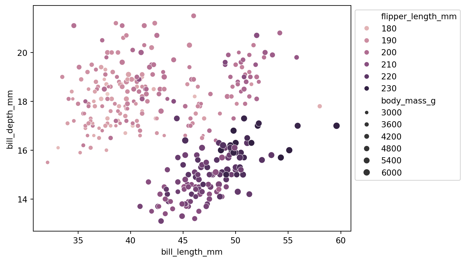
Note: Using transparency helps reveal point clustering, but if a gradient color is already used to differentiate a variable (as in Figure 14), transparency should not be applied.
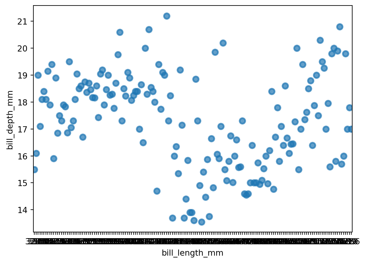
When a point plot uses ratio data as the x-axis, each point maps to a specific tick mark, as shown in Figure 11:
Note: Although the point distribution in Figure 10 and Figure 11 looks similar, each x-axis value in a point plot has exactly one corresponding point, while a scatter plot can have multiple. Also,
sns.pointplot()does not support adjusting point size, whilesns.scatterplot()does.
Therefore, point plots are not suitable when the x-axis is continuous data with too many tick marks; they work best when the x-axis is discrete data with a limited number of categories. Scatter plots are the opposite — better suited for ratio-ratio data.
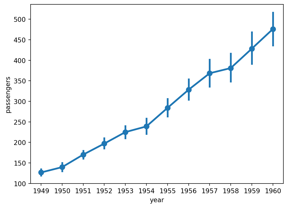
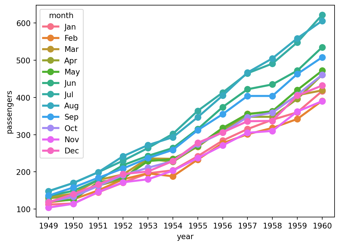
Another feature of point plots is that points can be connected with lines, which is appropriate when the x-axis uses ordinal or interval data. For example, in Figure 12, year is interval data and the connecting lines show passenger trends over time; in Figure 7, the x-axis represents penguin species (nominal data) where order is meaningless, so lines are not drawn.
This type of point plot becomes very similar to a line plot, which we will continue to discuss in Line Plot.
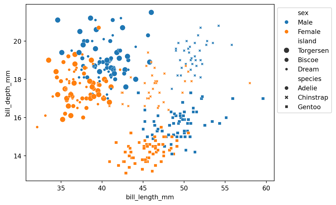
In addition to the two continuous variables on the x and y axes, other variables can be introduced by setting parameters such as hue (point color), size (point size), and style (point shape). hue and size can be applied to either continuous or discrete variables; style can only be applied to discrete variables, because point shapes cannot vary continuously (in Seaborn).
For example, Figure 13 introduces three discrete variables simultaneously:
In Figure 13, in addition to the two continuous variables on the axes (bill length and bill depth), three discrete variables are encoded (sex, island, and species). Similarly, Figure 14 introduces two continuous variables:
Note: Although
hueandsizecan be applied to continuous variables, their legends are not strictly continuous.
See Table 1 for a comparison of multivariate scatter plots and facet grids:
| Dimension | Multivariate Scatter Plot | Facet Grid |
|---|---|---|
| View | Global, all points in one coordinate system | Split into panels for easy subplot comparison |
| Space | Compact, only one chart needed | Larger, requires multiple subplots |
| Continuous variables | Can be added directly with auto-generated legend | Requires manual binning into a new discrete variable |
| Visual complexity | Information concentrated, may feel crowded | Each subplot is independent, lower reading burden |
| Legend reliance | Requires repeatedly consulting the legend | Subplot titles explain directly |
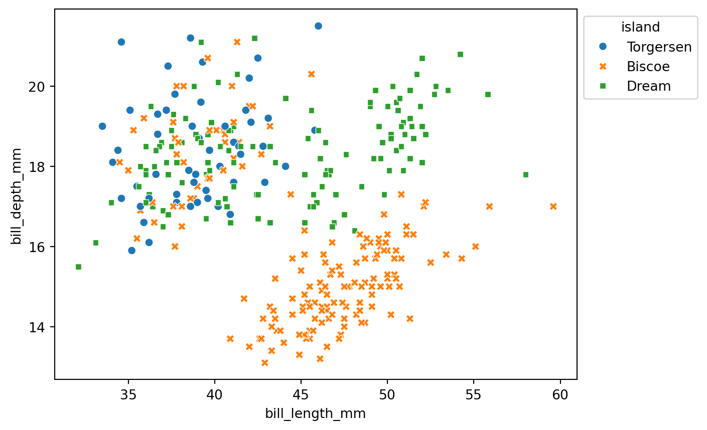
To make scatter plots easier to read, it is recommended to use both color and shape to distinguish the same variable (Wilke, 2019, pp.243-247), as in Figure 15:
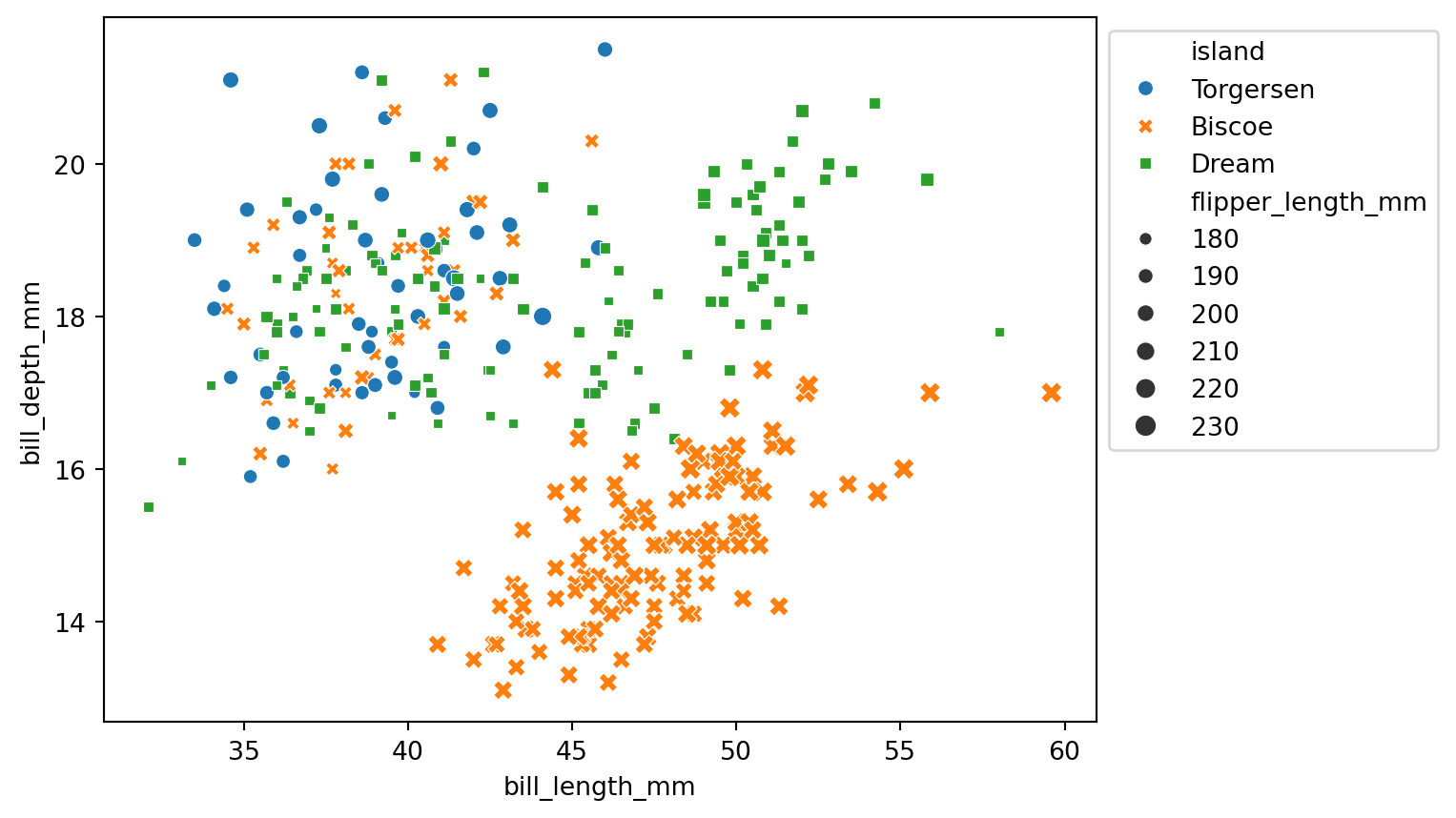
Furthermore, avoid using both style and size to control two different variables in the same chart, because when shapes differ, size differences become harder to perceive (see Figure 16):
Other notes:
These details will be further discussed in Section 4.
A logarithmic scale is a nonlinear measurement scale used for data with a wide range of values, such as the Richter scale, acoustic volume, optical intensity, and solution pH. When plotting such data, the axis can be set to a logarithmic scale (the default is a linear scale — for example, the x-axis tick marks 35, 40, 45, 50 in Figure 10 increase linearly), making otherwise crowded data points more evenly distributed and easier to observe (Wikipedia - Logarithmic scale).
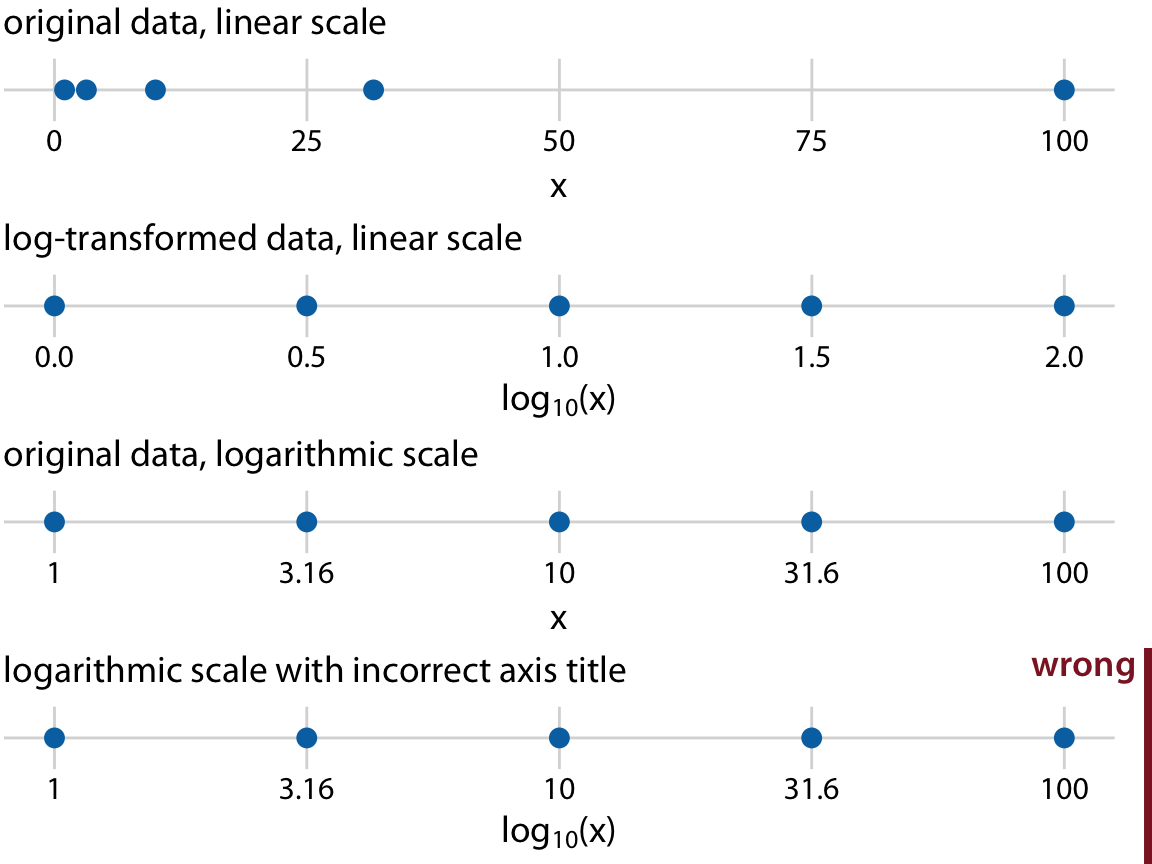
Wilke (2019, p.17) uses \((1, 3.16, 10, 31.6, 100)\) as an example to illustrate four number lines (Figure 17), where \(10^{0.5} = \sqrt{10} \approx 3.16\) and \(10^{1.5} \approx 31.6\).
As shown in Figure 17, the four number lines are interpreted as follows:
Comparing the first and third number lines: for the same data, points that are unevenly distributed on a linear scale become evenly distributed on a logarithmic scale. This adjustment helps observe data that is unevenly distributed, especially data following an exponential growth trend.
Note that switching to a logarithmic scale only changes how the axis tick marks are displayed — it does not change the values of the data points. Therefore, for a chart that only changes the scale without modifying the original data, the axis title must not be written as \(\log_{10}(x)\) (see the fourth number line).
When to use a logarithmic scale and its trade-offs:
When to use
Advantages
Disadvantages
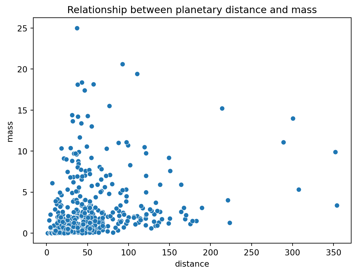
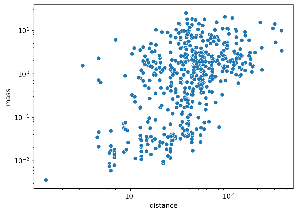
For example, Figure 18 shows data with a large range that is too concentrated on the left — switching to a logarithmic scale (Figure 19) improves the distribution.
Note: In Figure 19, the tick marks \((10^0, 10^1, 10^2, ...)\) are evenly spaced on a logarithmic scale. The minor tick marks between each pair of major tick marks represent linearly spaced actual values — for example, between \(10^0\) and \(10^1\) they are \(2, 3, ..., 9\), and between \(10^1\) and \(10^2\) they are \(20, 30, ..., 90\), and so on.
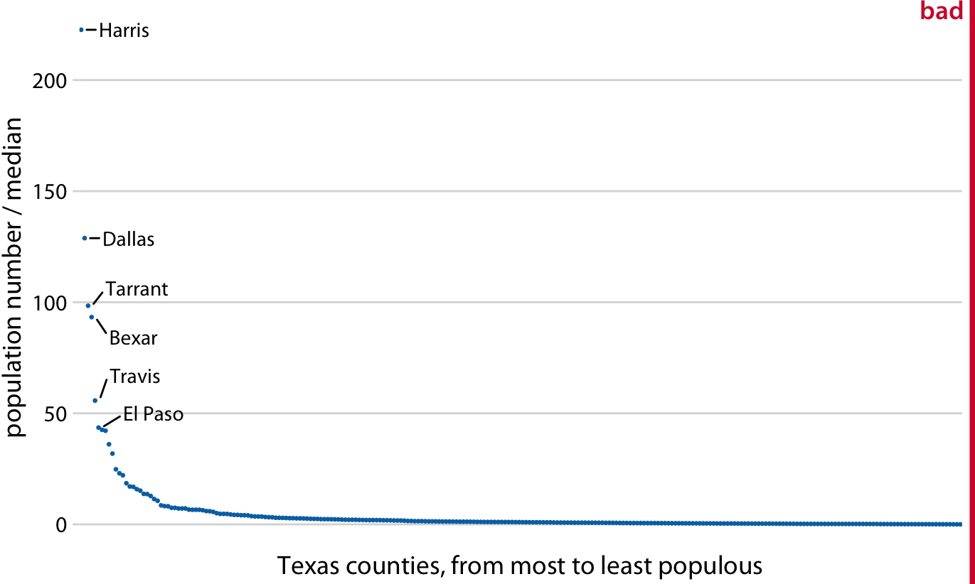
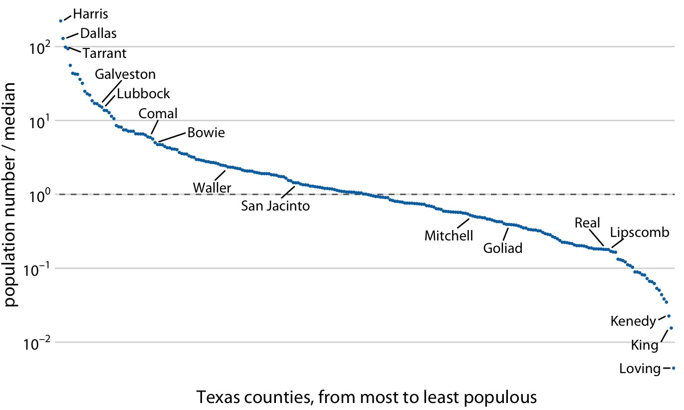
Because a logarithmic scale has no zero (with 1, i.e., the base raised to the power of 0, as the origin), a logarithmic scale is well suited for displaying ratio data. For example, Wilke (2019, pp.18-20) divides each county’s population in Texas by the median population as the y-axis, using a logarithmic scale (Figure 20) to show how each county’s population is distributed around the median (a ratio of 1 means the county’s population equals exactly the median).
If the data in Figure 20 were displayed with a linear scale, the origin would be 0, making it impossible to clearly show the distribution of values around 1 (Figure 21).
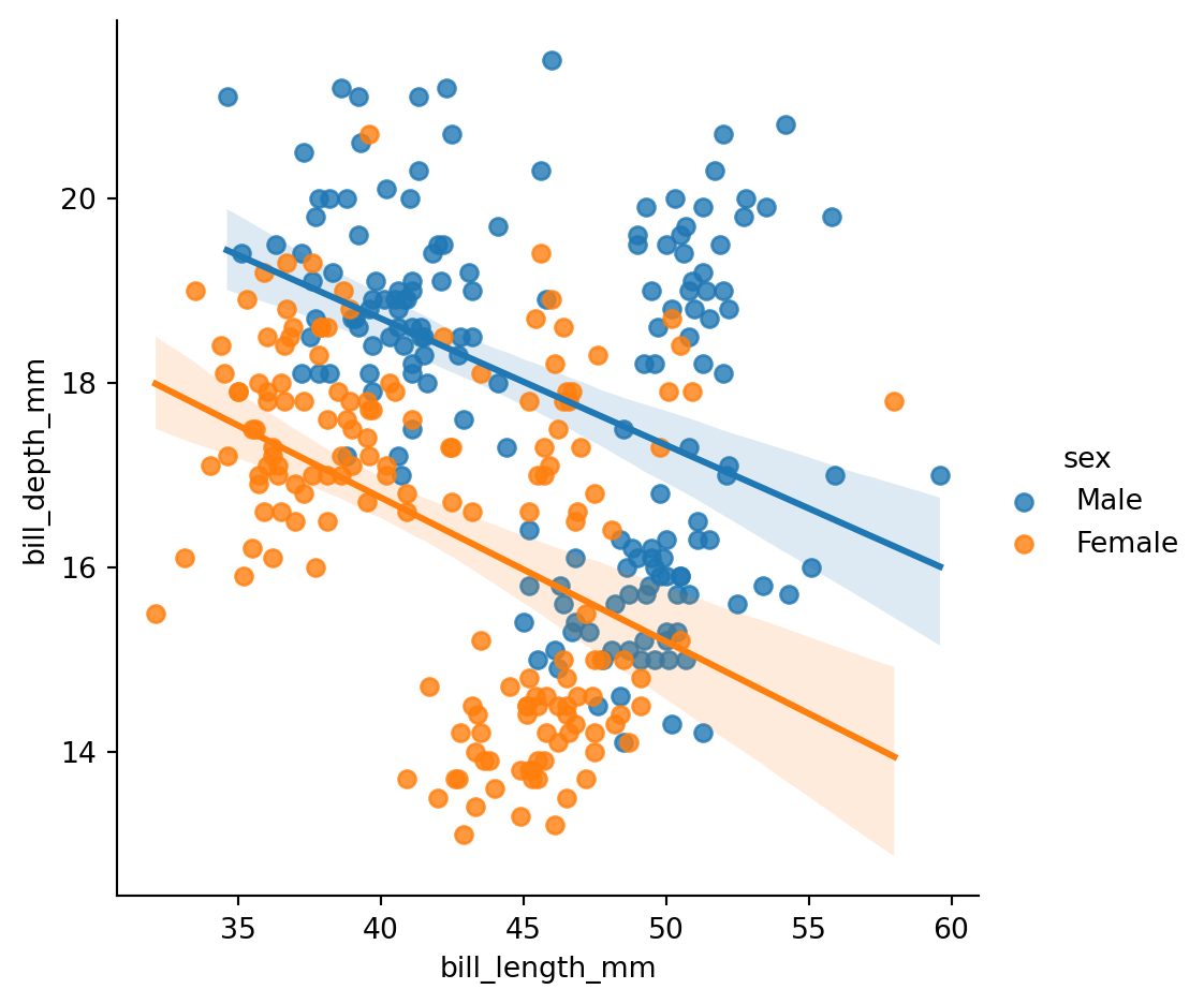
A regression plot fits the scatter plot to a line, showing the relationship between two variables. The most common is linear fitting, which fits a linear regression line to the scatter plot. The confidence interval shows the uncertainty of the regression line (as an estimate): at a 95% confidence level, the true value has a 95% chance of falling within that interval. In Figure 22, the line is the linear regression line and the shaded area is the confidence interval.
sns.lmplot() (linear model plot) uses a 95% confidence interval by default to measure the uncertainty of the regression line.
Note: The
hueparameter only works with discrete data.
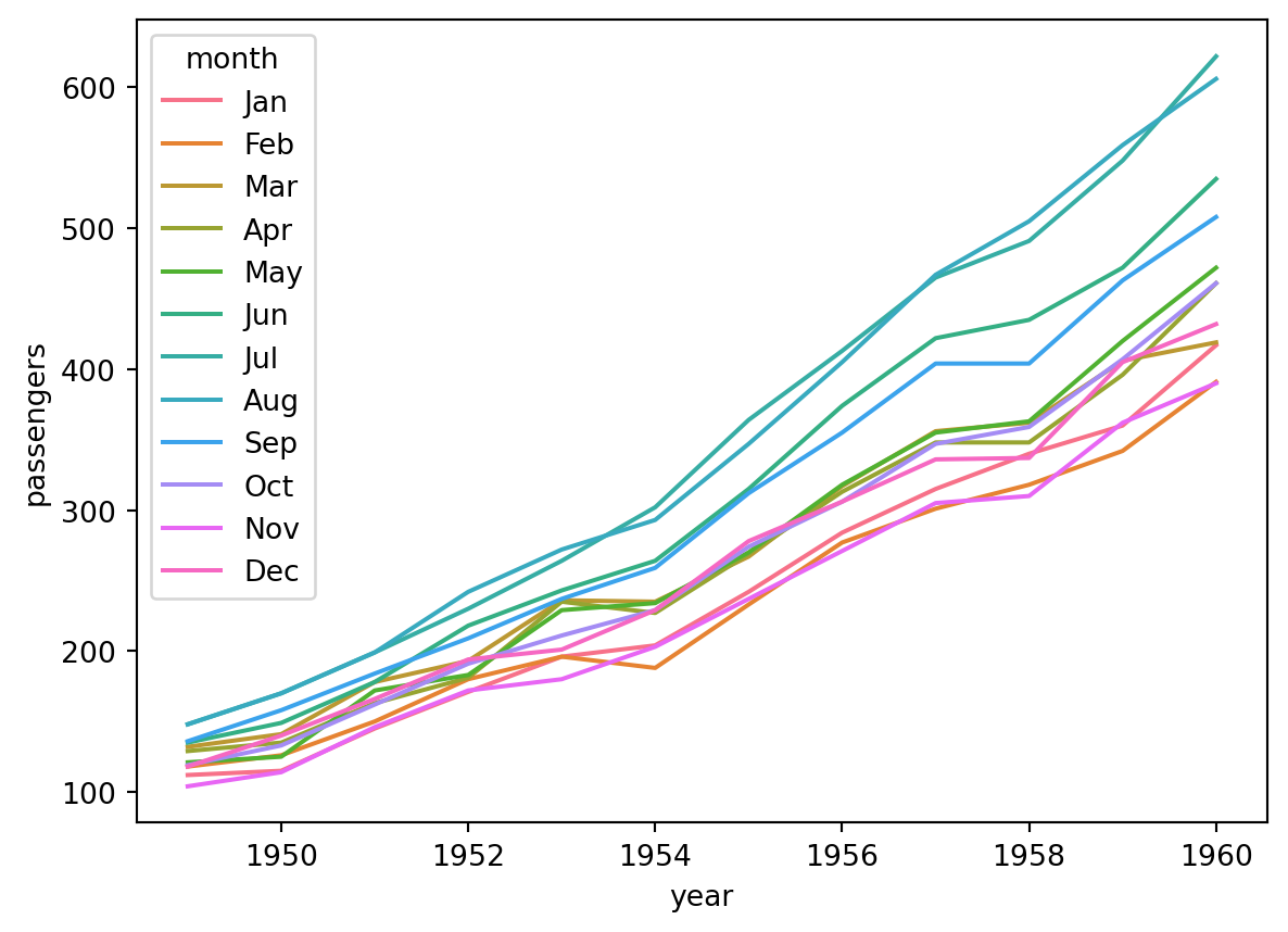
In a scatter plot, data points exist independently and are typically used to explore the correlation or distribution between two variables, with no inherent ordering among data points. In a line plot, data points are connected by line segments to emphasize continuity or trend, typically used for time-series data to show how one variable changes over time, where data points have an inherent ordering.
For example, Figure 23 shows how monthly passenger counts for an airline change over the years:
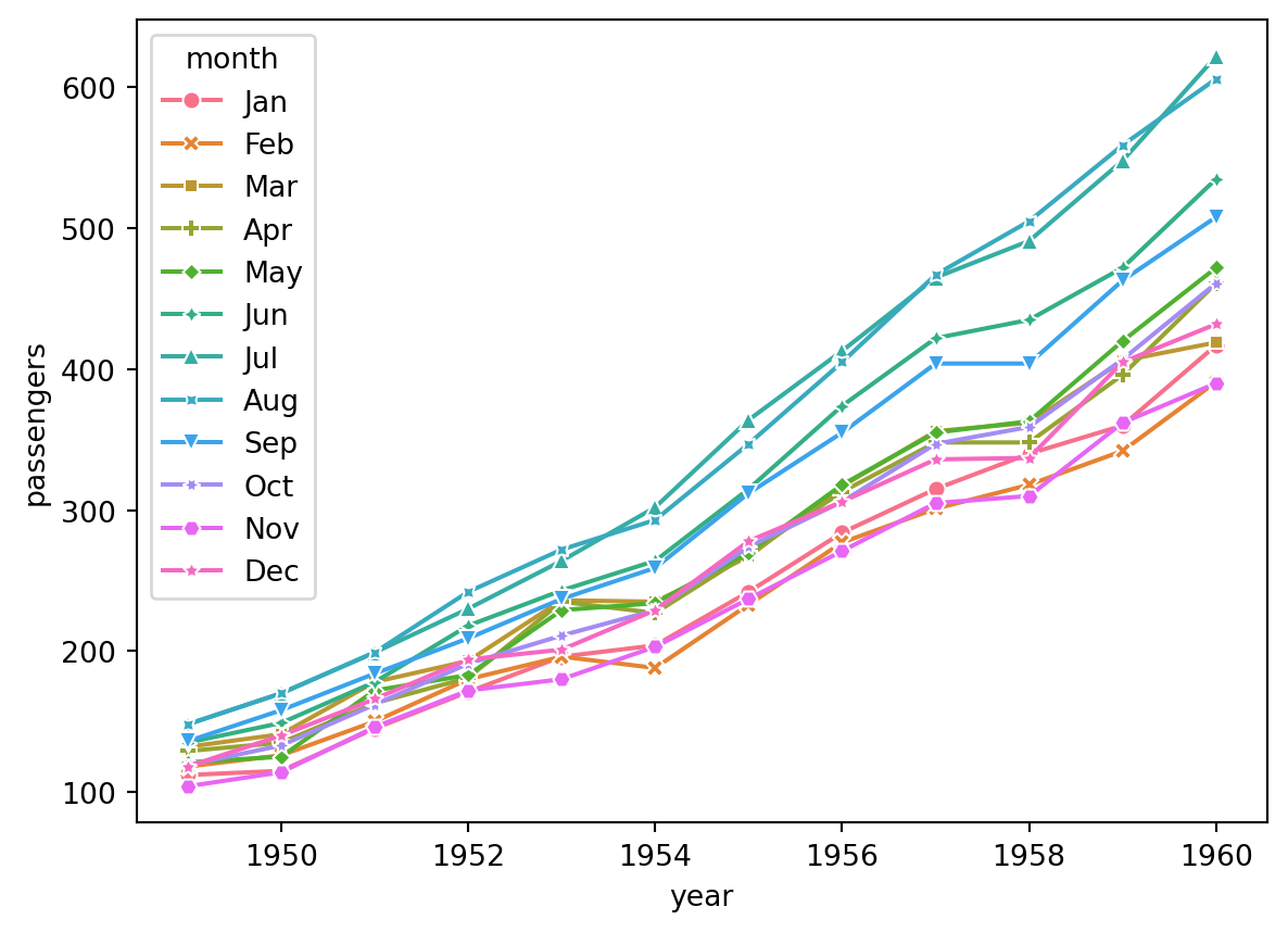
You can also display markers by setting markers=True and dashes=False (Figure 24):
When there are many data points, it is not recommended to display markers in a line plot — too many markers impede readability; clean lines better convey the trend (Wilke, 2019, pp. 135-137).
A similar effect can be achieved with a point plot (see Figure 25), but sns.pointplot() cannot use different marker shapes to distinguish variables and cannot remove markers, so sns.lineplot() is the better choice for observing trends over time.
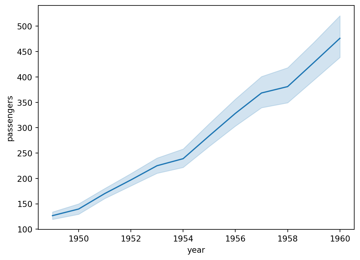
When the y-axis variable has multiple values at each time point and no color distinction is applied, sns.lineplot() automatically generates a mean line and error band (default 95% confidence level), see Figure 26:
When using color to distinguish lines in a line plot, note:
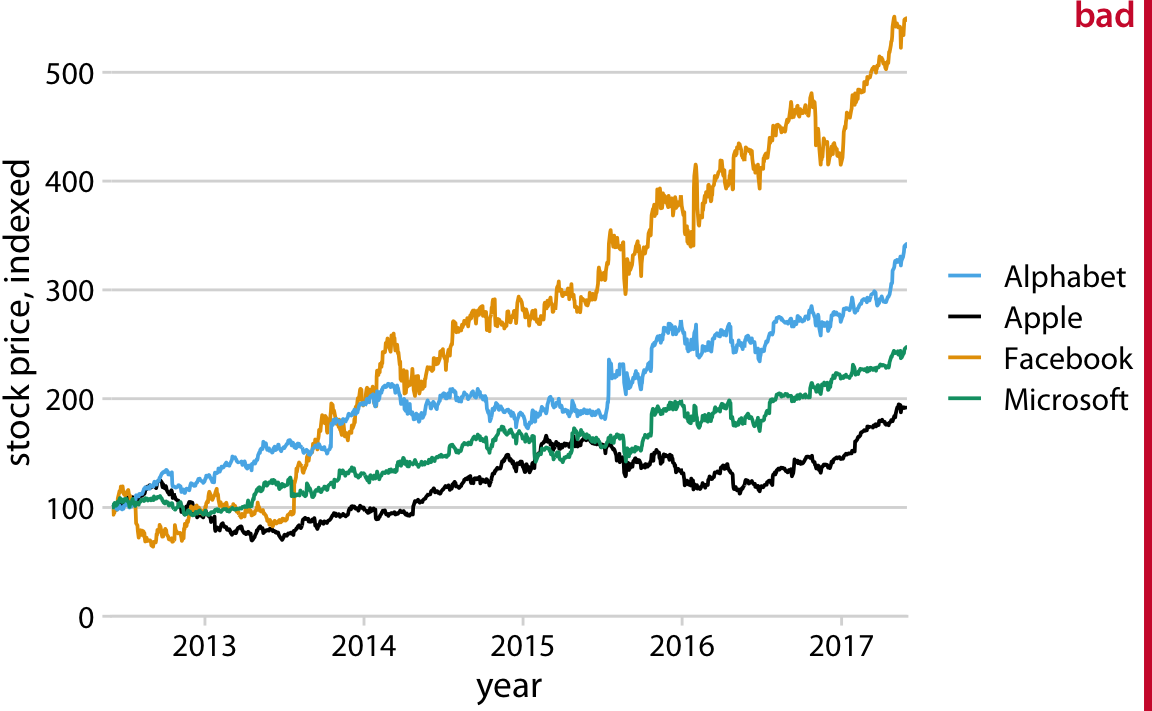
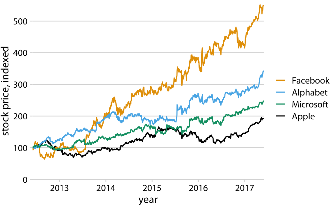
In Figure 27, the legend and line color orders are inconsistent, which increases reading difficulty. Wilke (2019, p.248) provides a counter-example:
In contrast, Figure 28 has matching legend and line color orders. Wilke (2019, p.249) provides the improved chart:
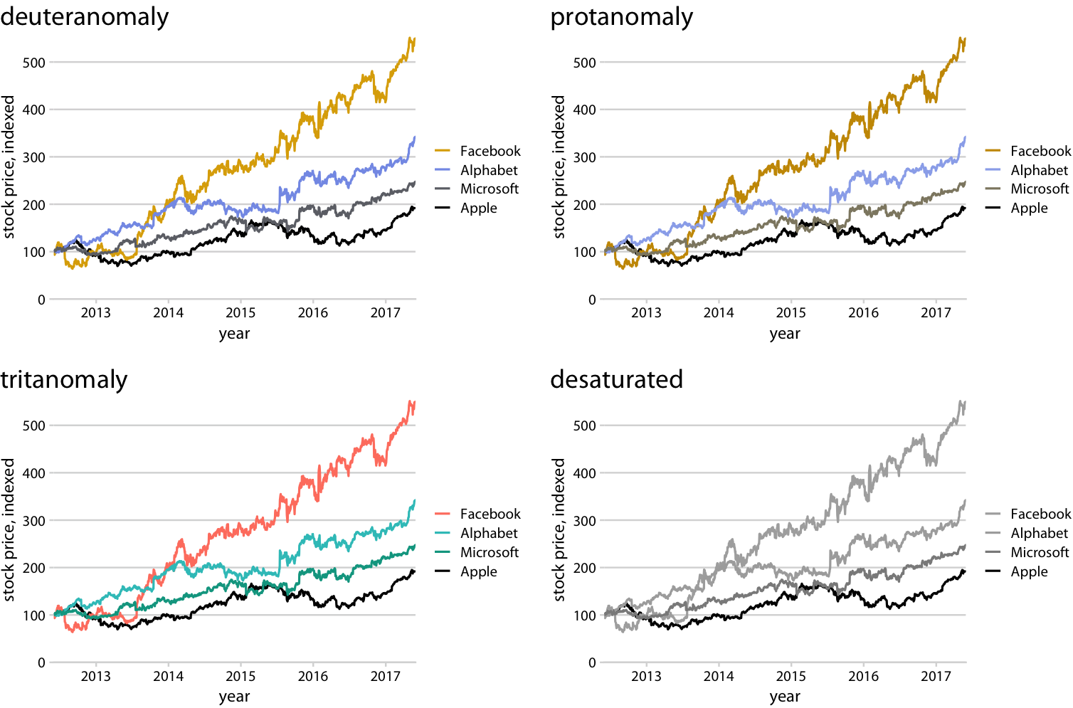
Wilke (2019, p.250) also shows how Figure 28 appears under simulations of different color vision deficiencies and after desaturation (Figure 29):
From Figure 29, the color scheme in Figure 28 is distinguishable for all three types of color vision deficiencies, and remains distinguishable by lightness after desaturation. This is why matching legend and line color order is especially important.
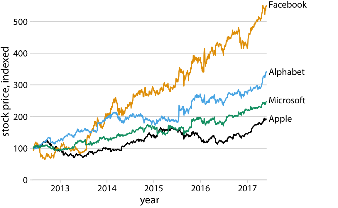
Additionally, Wilke (2019, p.251) recommends removing the legend and labeling each line directly (Figure 30), which saves readers the effort of consulting a legend and makes the chart easier to read. However, this is difficult to implement in Seaborn, so in this course it is sufficient to use a legend with colors in the correct order as in Figure 28.
Before creating a heatmap, the original data must first be reshaped into a pivot table. A pivot table presents two variables from the original table in matrix form: column names represent one variable and row names represent the other.
The pivot operation converts all unique values in a column of the original table into new column labels or row indices. For example, Table 3 converts all unique values of the 'year' column in Table 2 (1949–1960) into new column names, and the unique values of the 'month' column into row names.
The pivot and melt operations are opposites: pivot converts a “long” table into a “wide” table, while melt converts a “wide” table into a “long” table (melt turns column names into data values, increasing the number of rows).
| year | month | passengers | |
|---|---|---|---|
| 0 | 1949 | Jan | 112 |
| 1 | 1949 | Feb | 118 |
| 2 | 1949 | Mar | 132 |
| 3 | 1949 | Apr | 129 |
| 4 | 1949 | May | 121 |
# create pivot table (can also be named matrix)
flights_pivot = pd.pivot_table(
flights,
index='month', # unique values of 'month' become row index
columns='year', # unique values of 'year' become column names
values='passengers',
observed=False, # show all possible combinations of categorical variables
)
flights_pivot| year | 1949 | 1950 | 1951 | 1952 | 1953 | 1954 | 1955 | 1956 | 1957 | 1958 | 1959 | 1960 |
|---|---|---|---|---|---|---|---|---|---|---|---|---|
| month | ||||||||||||
| Jan | 112.0 | 115.0 | 145.0 | 171.0 | 196.0 | 204.0 | 242.0 | 284.0 | 315.0 | 340.0 | 360.0 | 417.0 |
| Feb | 118.0 | 126.0 | 150.0 | 180.0 | 196.0 | 188.0 | 233.0 | 277.0 | 301.0 | 318.0 | 342.0 | 391.0 |
| Mar | 132.0 | 141.0 | 178.0 | 193.0 | 236.0 | 235.0 | 267.0 | 317.0 | 356.0 | 362.0 | 406.0 | 419.0 |
| Apr | 129.0 | 135.0 | 163.0 | 181.0 | 235.0 | 227.0 | 269.0 | 313.0 | 348.0 | 348.0 | 396.0 | 461.0 |
| May | 121.0 | 125.0 | 172.0 | 183.0 | 229.0 | 234.0 | 270.0 | 318.0 | 355.0 | 363.0 | 420.0 | 472.0 |
| Jun | 135.0 | 149.0 | 178.0 | 218.0 | 243.0 | 264.0 | 315.0 | 374.0 | 422.0 | 435.0 | 472.0 | 535.0 |
| Jul | 148.0 | 170.0 | 199.0 | 230.0 | 264.0 | 302.0 | 364.0 | 413.0 | 465.0 | 491.0 | 548.0 | 622.0 |
| Aug | 148.0 | 170.0 | 199.0 | 242.0 | 272.0 | 293.0 | 347.0 | 405.0 | 467.0 | 505.0 | 559.0 | 606.0 |
| Sep | 136.0 | 158.0 | 184.0 | 209.0 | 237.0 | 259.0 | 312.0 | 355.0 | 404.0 | 404.0 | 463.0 | 508.0 |
| Oct | 119.0 | 133.0 | 162.0 | 191.0 | 211.0 | 229.0 | 274.0 | 306.0 | 347.0 | 359.0 | 407.0 | 461.0 |
| Nov | 104.0 | 114.0 | 146.0 | 172.0 | 180.0 | 203.0 | 237.0 | 271.0 | 305.0 | 310.0 | 362.0 | 390.0 |
| Dec | 118.0 | 140.0 | 166.0 | 194.0 | 201.0 | 229.0 | 278.0 | 306.0 | 336.0 | 337.0 | 405.0 | 432.0 |
About the aggfunc parameter. The aggfunc (aggregation function) in pd.pivot_table() defaults to 'mean', meaning when a single cell corresponds to multiple rows in the original data, it takes the mean by default.
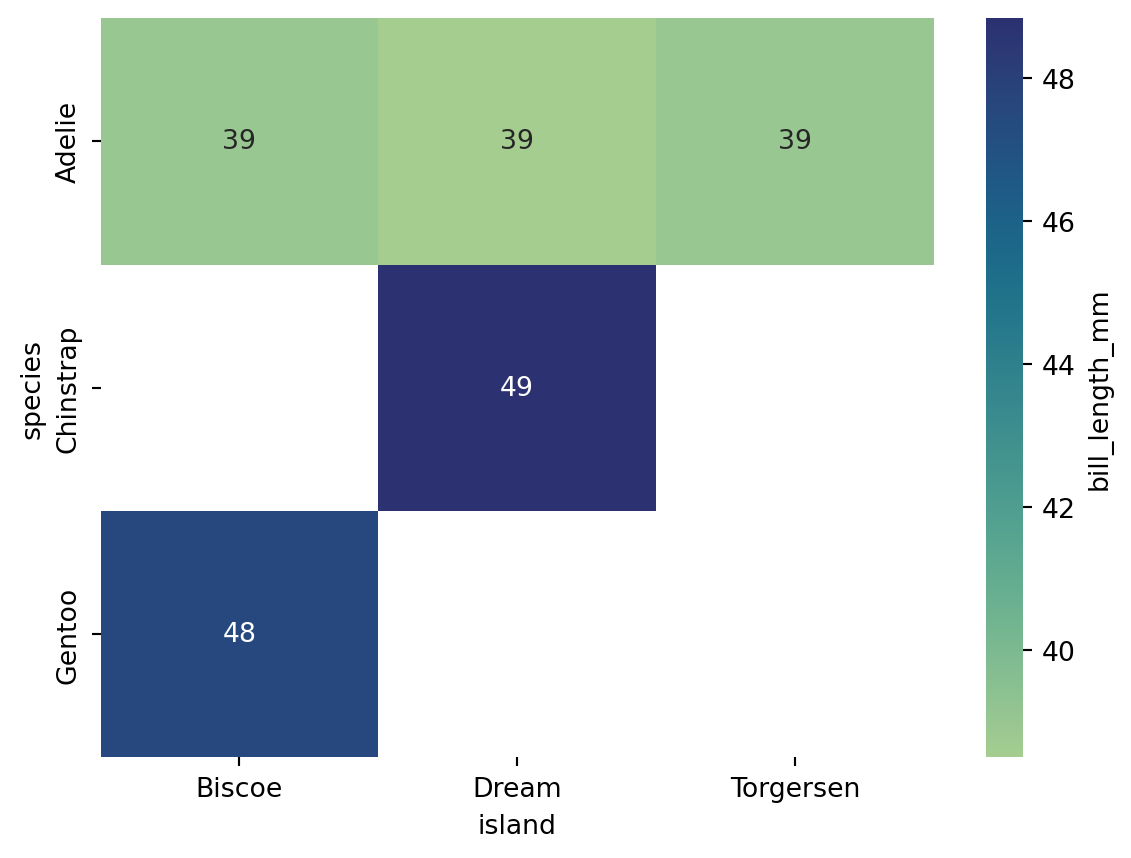
In Table 2, each combination of year and month has only one passenger value, so no averaging is needed. However, in the penguin dataset shown in Table 4, there is more than one penguin per species-island combination, and each combination maps to a single cell in the pivot table (Table 5), so the default mean is applied.
| species | island | bill_length_mm | bill_depth_mm | flipper_length_mm | body_mass_g | sex | |
|---|---|---|---|---|---|---|---|
| 0 | Adelie | Torgersen | 39.1 | 18.7 | 181.0 | 3750.0 | Male |
| 1 | Adelie | Torgersen | 39.5 | 17.4 | 186.0 | 3800.0 | Female |
| 2 | Adelie | Torgersen | 40.3 | 18.0 | 195.0 | 3250.0 | Female |
| 3 | Adelie | Torgersen | NaN | NaN | NaN | NaN | NaN |
| 4 | Adelie | Torgersen | 36.7 | 19.3 | 193.0 | 3450.0 | Female |
| island | Biscoe | Dream | Torgersen |
|---|---|---|---|
| species | |||
| Adelie | 38.975000 | 38.501786 | 38.95098 |
| Chinstrap | NaN | 48.833824 | NaN |
| Gentoo | 47.504878 | NaN | NaN |
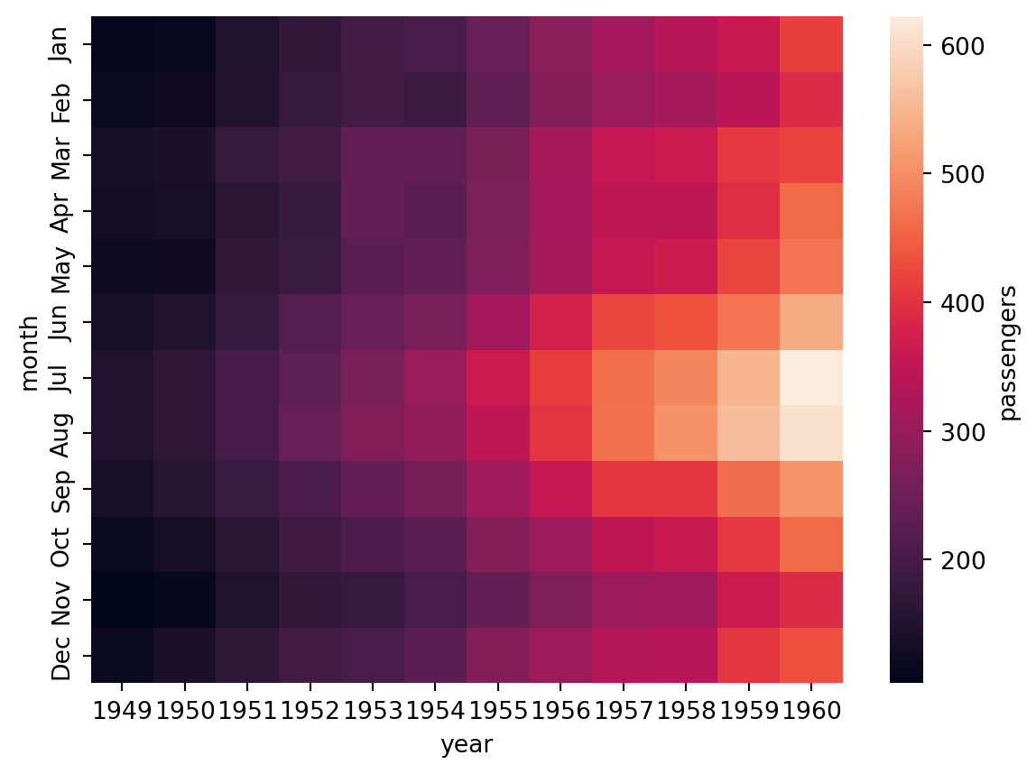
Using Table 3 to create a heatmap, see Figure 31:
.heatmap plots directly from a matrix-shaped table, rather than specifying particular columns through x/y parameters. cbar_kws (colorbar keyword arguments) sets the label for the colorbar.
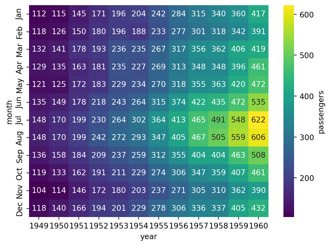
Additional parameters such as cmap and annot can be used to further customize the heatmap (Figure 32):
cmap accepts the name of a predefined color palette or colormap from Seaborn or Matplotlib, such as 'crest', 'flare', 'viridis', or 'pink'.
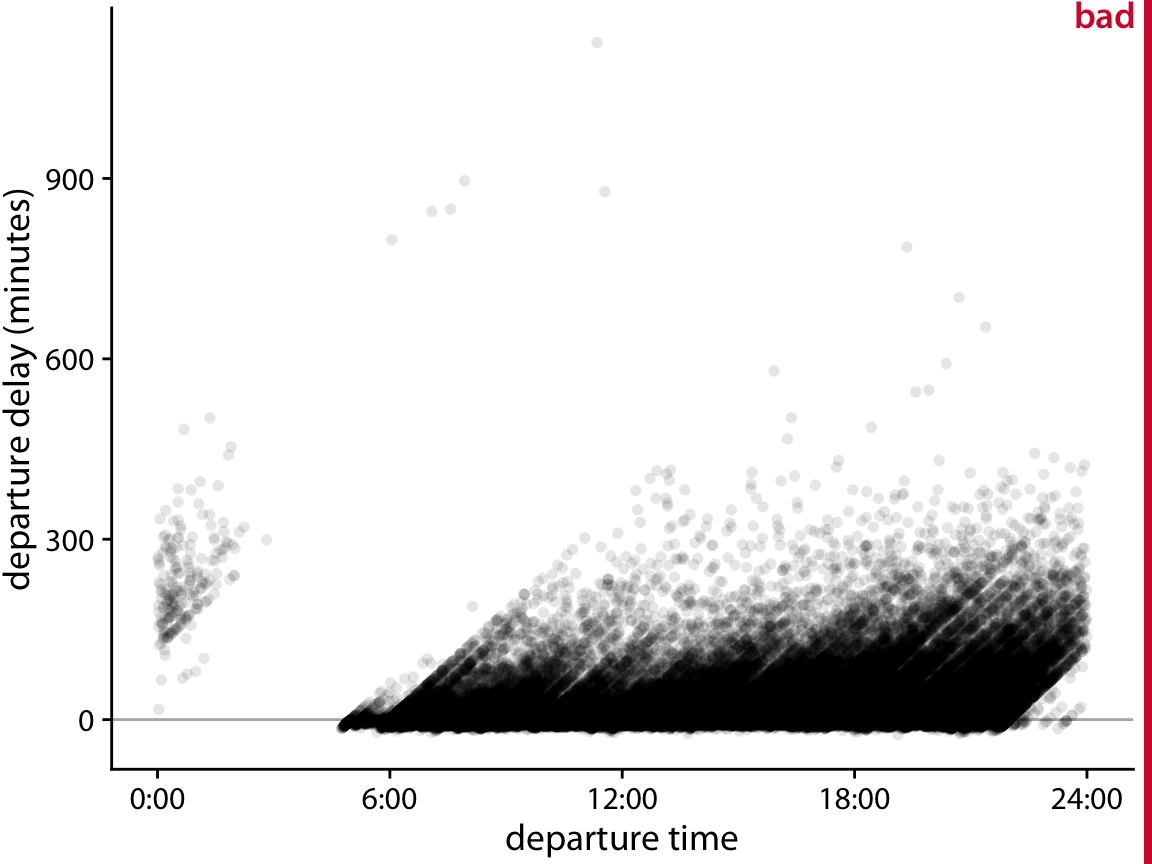
According to Wilke (2019, pp. 222-225), scatter plots with semi-transparent points can show the distribution of data across two variables, but when data points are too numerous and dense, a scatter plot struggles to convey the overall distribution (see Figure 34: high-density areas appear as uniform dark blotches while low-density areas are nearly invisible).
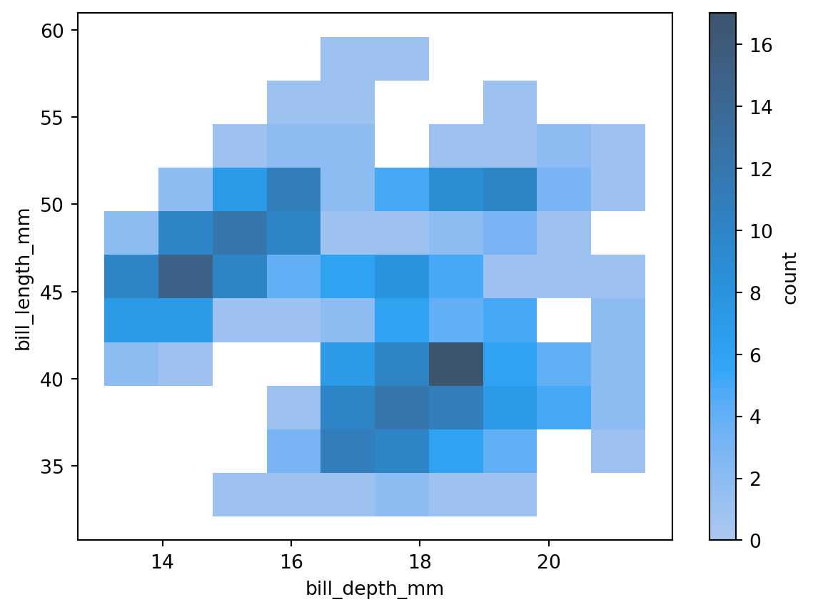
In such cases, a 2D histogram can be used instead: the x-y plane is divided into small rectangles (bins), the number of data points falling into each bin is counted, and each rectangle is colored according to that count (see Figure 35):
Table 6 shows the differences between heatmaps and 2D histograms:
| Property | Heatmap | 2D Histogram |
|---|---|---|
| Input data | Pre-processed matrix (usually from a pivot table) | Raw data |
| Axes | Usually represent two discrete variables | Usually represent two continuous variables |
| Number of variables | Three: axes and color | Two: axes only |
| Color meaning | Magnitude of the value in each cell | Number of data points in each bin |
| Layout | Fixed rows and columns, fixed color-value mapping | Shape can vary depending on the number of bins |
| Main use | Show numerical patterns in a matrix | Show the joint distribution density of two variables |
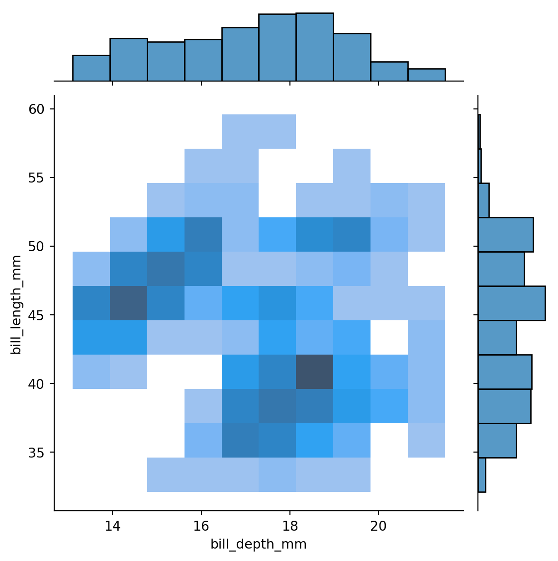
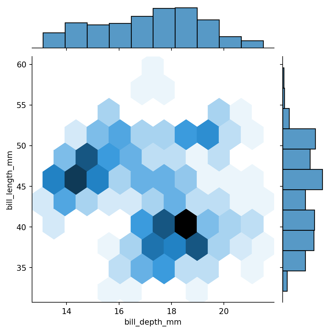
sns.jointplot() can simultaneously display the bivariate distribution of two variables along with their individual univariate distributions.
As shown in Figure 36, you can display a 2D histogram (same as Figure 35) while also showing the 1D histogram of each variable:
You can also set kind='hex' to use hexagonal bins in the center panel (Figure 37):
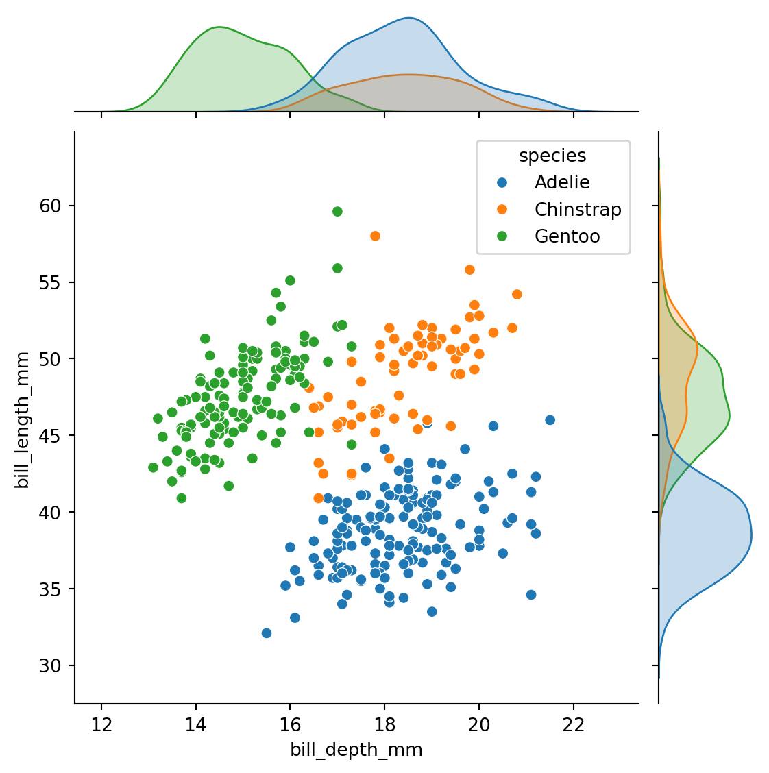
Color can also be used to distinguish variables (Figure 38):
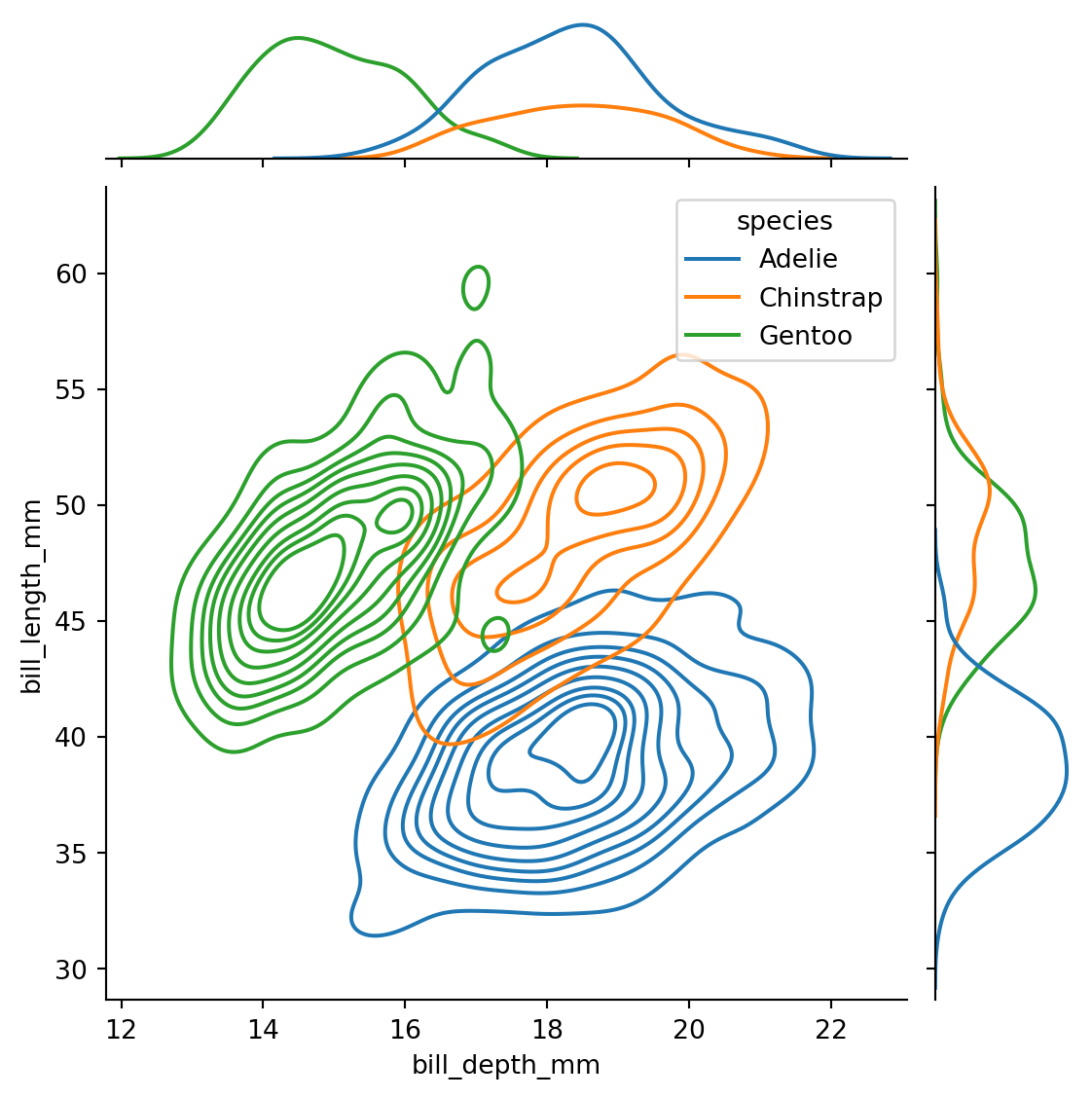
You can also use kind='kde' (kernel density estimation) to generate smoothed distribution curves (see Figure 39). However, smoothed curves are not actual data and can mislead readers, especially when there are few data points, so they are not recommended in this course.
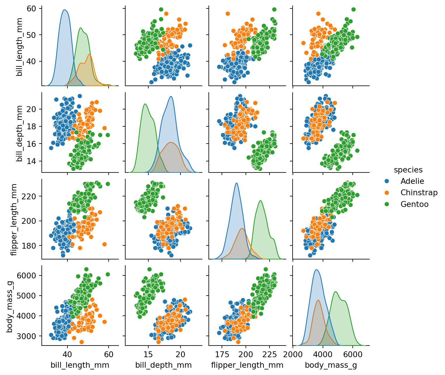
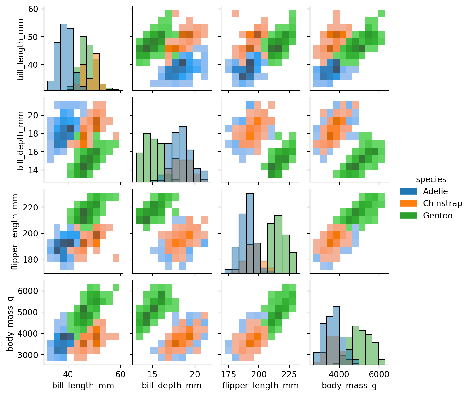
sns.pairplot() makes it easy to plot pairwise distributions for multiple variables (i.e., multiple columns) in the original dataset, forming a grid of plots (Figure 40):
In Figure 40, the four ratio variables in the original DataFrame are automatically detected and plotted: the diagonal plots are the univariate distributions of each variable, while the remaining subplots are bivariate distributions based on each pair of variables.
You can also modify the format of the diagonal and off-diagonal plots using diag_kind and kind (Figure 41):
---
title: 'Multivariate Plots'
author: 'Pinn Xu'
date: '2024-10-27'
# categories: ["Python", "Visualization", "Multivariate", "FacetGrid", "Heatmap", "Joint Plot", "Pair Plot"]
categories: ["Python", "FacetGrid", "Heatmap"]
description: 'Use Seaborn to create multivariate visualizations: scatter plots, line pots, heatmaps, joint plots, facet grids, etc.'
code-fold: false
number-sections: true
image: ../../../src/img/ttl/multi/cover.png
order: 3
aliases:
- ../multivariate-plots/
---
```{python}
#| eval: false
#| code-fold: true
#| code-summary: "Environment and Versions"
python==3.12
pandas==2.2.2
matplotlib==3.9.x
seaborn==0.13.2
```
# Multivariate Data
**"Tidy/flat" tabular data:** Each row is one **observation** (also called instance or record), and each column is one **variable** (also called attribute, feature, or parameter).
Typically, **multivariate** refers to data with more than two variables — a multivariate plot generally uses three or more columns from the original DataFrame.
When creating a bar chart, in addition to the x and y variables, you can also set the `hue` parameter to include a third variable. For example, @fig-bar-variables includes three variables: `'island'`, `'body_mass_g'`, and `'sex'`.
```{python}
# import libraries
import pandas as pd
import seaborn as sns
import matplotlib.pyplot as plt
```
```{python}
# load example dataset from Seaborn
df = sns.load_dataset('penguins')
```
```{python}
#| label: fig-bar-variables
#| fig-cap: "Bar chart with three variables"
sns.barplot(df, x='island', y='body_mass_g', hue='sex')
plt.show()
```
However, some chart types do not support setting `x`, `y`, and `hue` all at once. For example, a histogram only supports `x` and `hue` (see @fig-histogram-variables): the x-axis shows distribution intervals of flipper length, and the y-axis shows the number of penguins in each interval, involving only two variables.
```{python}
#| label: fig-histogram-variables
#| fig-cap: "Histogram with two variables"
sns.histplot(data=df, x='flipper_length_mm', hue='island')
plt.show()
```
# Facet Grid
A facet grid (FacetGrid) is a common method for displaying multivariate data. Several small charts (facets) are arranged in a grid to form a facet grid. If you want to display a histogram while also showing more than two variables, you can use a facet grid.
The method for creating a facet grid with Seaborn is as follows:
```{python}
#| label: fig-empty-facetgrid
#| fig-cap: "Empty 3×2 facet grid"
# create an empty facet grid
g = sns.FacetGrid(
data=df,
col='sex', # creates one column per unique value of 'sex'
row='island', # 'island' has three values, creating three rows
)
plt.show()
```
As shown in @fig-empty-facetgrid, we created a 3×2 facet grid, but it is currently empty. Use the `.map_dataframe()` method to specify the content to fill in.
```{python}
#| label: fig-filled-facetgrid
#| fig-cap: "Filled facet grid"
# fill the complete facet grid
# Step 1: create facet grid
g = sns.FacetGrid(
data=df,
col='sex',
row='island',
hue='species',
)
# Step 2: fill with histograms
g.map_dataframe(
sns.histplot,
x='flipper_length_mm',
stat='density', # sum of bar areas equals 1 for each group
common_norm=False, # each color normalized independently within each facet
)
# Step 3: add and adjust legend
g.add_legend()
sns.move_legend(
g,
loc='lower center',
bbox_to_anchor=(0.5, 1),
ncol=3, # number of legend columns
)
plt.show()
```
**stat and common_norm**
`stat='density'` uses frequency density for plotting, so the total area of all bars in the histogram sums to 1. `common_norm=False` is used alongside `stat`, meaning each color's bars within the same facet are normalized independently, rather than all colors being normalized together.
**loc and bbox_to_anchor**
Setting both parameters together positions the lower-center edge of the legend at coordinates (0.5, 1) of the entire grid figure. If only `loc='lower center'` is set, the legend will be placed at the lower center of the grid figure directly.
As shown in @fig-filled-facetgrid, the facet grid separates rows by island, columns by sex, and colors by species, simultaneously displaying four variables (flipper length, island, sex, species). Splitting by rows and columns allows two additional discrete variables; color differentiation can add one more discrete variable.
> Note: Because of how rows and columns work, facet grids can only add discrete variables. To facet by a continuous variable, first bin it into intervals and save as a new discrete variable column, then use the facet grid for row or column splitting.
**Consistent Axis Ranges**
When displaying multiple subplots together, each subplot should have the same axis range, because readers tend to assume that axis ranges are consistent across panels — inconsistency can lead to misinterpretation [(Wilke, 2019, pp. 257-258)](https://clauswilke.com/dataviz/multi-panel-figures.html#small-multiples).
In @fig-ba-degrees-variable-y-lims, each subplot has a different y-axis range, which is easy to misread. Changing to @fig-ba-degrees-fixed-y-lims with consistent axis ranges across all subplots reduces reading difficulty.
[{#fig-ba-degrees-variable-y-lims fig-alt="Bad multi-panel axis ranges (Wilke, 2019, p. 258)"}](https://clauswilke.com/dataviz/multi-panel-figures.html#fig:BA-degrees-variable-y-lims)
[{#fig-ba-degrees-fixed-y-lims fig-alt="Improved multi-panel axis ranges (Wilke, 2019, p. 259)"}](https://clauswilke.com/dataviz/multi-panel-figures.html#fig:BA-degrees-fixed-y-lims)
# Scatter Plot
## Distinguishing Scatter Plots from Point Plots
Before creating scatter plots, it is important to distinguish between **scatter plots** and **point plots**.
> Note: Point plots are also called dot plots [(Wilke, 2019, p.43)](https://clauswilke.com/dataviz/directory-of-visualizations.html#directory-uncertainty). The following distinction between scatter plots and point plots is based on the Seaborn library and may differ in other contexts.
**A point plot** can function similarly to a bar chart: the vertical line at each point is equivalent to a bar in a bar chart, and the point corresponds to the midpoint of the top edge of each bar. Like a bar chart, a point plot can be used for category-amount charts (see @fig-pointplot-category-amount and @fig-barplot-category-amount):
```{python}
#| label: fig-pointplot-category-amount
#| fig-cap: "Point plot: penguin species vs. bill length (black lines are error bars)"
sns.pointplot(
data=df, x='species', y='bill_length_mm',
linestyles='none', # no lines connecting points
)
plt.show()
```
```{python}
#| label: fig-barplot-category-amount
#| fig-cap: "Bar chart: penguin species vs. bill length (black lines are error bars)"
sns.barplot(data=df, x='species', y='bill_length_mm')
plt.show()
```
As shown in @fig-pointplot-category-amount and @fig-barplot-category-amount, both point plots and bar charts can represent category-amount relationships. One key difference is that the amount axis in a bar chart must start at 0, while a point plot does not. Both point plots and bar charts only show the mean of the y-axis values (or other statistics such as the median), with each x-axis value corresponding to only one y-axis value.
**A scatter plot** displays every individual data point (see @fig-scatterplot-category-amount):
```{python}
#| label: fig-scatterplot-category-amount
#| fig-cap: "Scatter plot: category-amount (shows all data points, not averages)"
sns.scatterplot(data=df, x='species', y='bill_length_mm')
plt.show()
```
In a scatter plot, each x-axis value can correspond to multiple y-axis values, while in a point plot each x-axis value corresponds to only one y-axis value.
Scatter plots are commonly used to explore the relationship between two (or more) variables and to examine whether correlations exist, primarily between two continuous numeric variables. The x-axis of a scatter plot is therefore usually ratio data, with tick marks automatically displayed as a continuous numeric range (see @fig-scatterplot-ratio-ratio):
```{python}
#| label: fig-scatterplot-ratio-ratio
#| fig-cap: "Scatter plot: penguin bill length vs. bill depth (ratio-ratio)"
sns.scatterplot(
data=df, x='bill_length_mm', y='bill_depth_mm',
alpha=0.7, # semi-transparent to reveal point clustering
)
plt.show()
```
> Note: Using transparency helps reveal point clustering, but if a gradient color is already used to differentiate a variable (as in @fig-scatter-continuous-variables), transparency should not be applied.
When a **point plot** uses ratio data as the x-axis, each point maps to a specific tick mark, as shown in @fig-pointplot-ratio-ratio:
```{python}
#| label: fig-pointplot-ratio-ratio
#| fig-cap: "Point plot: ratio variable on x-axis"
sns.pointplot(
data=df, x='bill_length_mm', y='bill_depth_mm',
linestyle='none', errorbar=None, alpha=0.7,
)
plt.show()
```
> Note: Although the point distribution in @fig-scatterplot-ratio-ratio and @fig-pointplot-ratio-ratio looks similar, each x-axis value in a point plot has exactly one corresponding point, while a scatter plot can have multiple. Also, `sns.pointplot()` does not support adjusting point size, while `sns.scatterplot()` does.
Therefore, **point plots are not suitable when the x-axis is continuous data with too many tick marks**; they work best **when the x-axis is discrete data** with a limited number of categories. **Scatter plots** are the opposite — better suited for ratio-ratio data.
Another feature of point plots is that points can be connected with lines, which is appropriate when the x-axis uses ordinal or interval data. For example, in @fig-pointplot-interval-ratio, year is interval data and the connecting lines show passenger trends over time; in @fig-pointplot-category-amount, the x-axis represents penguin species (nominal data) where order is meaningless, so lines are not drawn.
This type of point plot becomes very similar to a line plot, which we will continue to discuss in [Line Plot](#sec-line-plot).
```{python}
#| label: fig-pointplot-interval-ratio
#| fig-cap: "Point plot: year vs. passenger count (interval-ratio)"
flights = sns.load_dataset('flights')
sns.pointplot(data=flights, x='year', y='passengers')
plt.show()
```
## Multivariate Scatter Plot
In addition to the two continuous variables on the x and y axes, other variables can be introduced by setting parameters such as `hue` (point color), `size` (point size), and `style` (point shape). `hue` and `size` can be applied to either continuous or discrete variables; `style` can only be applied to discrete variables, because point shapes cannot vary continuously (in Seaborn).
For example, @fig-scatter-discrete-variables introduces three discrete variables simultaneously:
```{python}
#| label: fig-scatter-discrete-variables
#| fig-cap: "Adding three discrete variables: hue & size & style"
ax = sns.scatterplot(
data=df, x='bill_length_mm', y='bill_depth_mm',
hue='sex',
size='island',
style='species',
)
sns.move_legend(ax, loc='upper left', bbox_to_anchor=(1, 1))
plt.show()
```
In @fig-scatter-discrete-variables, in addition to the two continuous variables on the axes (bill length and bill depth), three discrete variables are encoded (sex, island, and species). Similarly, @fig-scatter-continuous-variables introduces two continuous variables:
```{python}
#| label: fig-scatter-continuous-variables
#| fig-cap: "Adding two continuous variables: hue & size (gradient color used, avoid transparency)"
ax = sns.scatterplot(
data=df, x='bill_length_mm', y='bill_depth_mm',
hue='flipper_length_mm',
size='body_mass_g',
)
sns.move_legend(ax, loc='upper left', bbox_to_anchor=(1, 1))
plt.show()
```
> Note: Although `hue` and `size` can be applied to continuous variables, their legends are not strictly continuous.
See @tbl-scatter-vs-facetgrid for a comparison of **multivariate scatter plots and facet grids**:
| Dimension | Multivariate Scatter Plot | Facet Grid |
|:---|:---:|:---:|
| View | Global, all points in one coordinate system | Split into panels for easy subplot comparison |
| Space | Compact, only one chart needed | Larger, requires multiple subplots |
| Continuous variables | Can be added directly with auto-generated legend | Requires manual binning into a new discrete variable |
| Visual complexity | Information concentrated, may feel crowded | Each subplot is independent, lower reading burden |
| Legend reliance | Requires repeatedly consulting the legend | Subplot titles explain directly |
: Comparison of multivariate scatter plots and facet grids {#tbl-scatter-vs-facetgrid}
To make scatter plots easier to read, it is recommended to **use both color and shape to distinguish the same variable** [(Wilke, 2019, pp.243-247)](https://clauswilke.com/dataviz/redundant-coding.html#designing-legends-with-redundant-coding), as in @fig-scatter-hue-style-island:
```{python}
#| label: fig-scatter-hue-style-island
#| fig-cap: "hue+style both control the same variable (island)"
ax = sns.scatterplot(
data=df, x='bill_length_mm', y='bill_depth_mm',
hue='island',
style='island',
)
sns.move_legend(ax, loc='upper left', bbox_to_anchor=(1, 1))
plt.show()
```
Furthermore, **avoid using both `style` and `size` to control two different variables in the same chart**, because when shapes differ, size differences become harder to perceive (see @fig-scatter-size-flipper):
```{python}
#| label: fig-scatter-size-flipper
#| fig-cap: "hue+style control island, size controls flipper length separately"
ax = sns.scatterplot(
data=df, x='bill_length_mm', y='bill_depth_mm',
hue='island',
style='island',
size='flipper_length_mm',
)
sns.move_legend(ax, loc='upper left', bbox_to_anchor=(1, 1))
plt.show()
```
**Other notes:**
- When using color, try to accommodate color-vision-impaired readers by choosing colors with **clearly distinct differences in both hue and lightness**.
- When there are too many data points, it is not recommended to display markers in a line plot.
These details will be further discussed in @sec-line-plot.
## Logarithmic Scale
**A logarithmic scale** is a nonlinear measurement scale used for data with a wide range of values, such as the Richter scale, acoustic volume, optical intensity, and solution pH. When plotting such data, the axis can be set to a logarithmic scale (the default is a linear scale — for example, the x-axis tick marks 35, 40, 45, 50 in @fig-scatterplot-ratio-ratio increase linearly), making otherwise crowded data points more evenly distributed and easier to observe ([Wikipedia - Logarithmic scale](https://en.wikipedia.org/wiki/Logarithmic_scale)).
[Wilke (2019, p.17)](https://clauswilke.com/dataviz/coordinate-systems-axes.html#nonlinear-axes) uses $(1, 3.16, 10, 31.6, 100)$ as an example to illustrate four number lines (@fig-linear-log-scales), where $10^{0.5} = \sqrt{10} \approx 3.16$ and $10^{1.5} \approx 31.6$.
[{#fig-linear-log-scales fig-alt="Four number lines (Wilke, 2019, p.17)" width="80%"}](https://clauswilke.com/dataviz/coordinate-systems-axes.html#fig:linear-log-scales)
As shown in @fig-linear-log-scales, the four number lines are interpreted as follows:
- **The first number line** uses a linear scale with tick marks at $(0, 25, 50, 75, 100)$, displaying the original data $x$. The data points are unevenly distributed.
- **The second number line** also uses a linear scale, but applies a logarithm to the data, displaying $\log_{10}(x)$. Data points are evenly distributed, with axis labels showing $\log_{10}(x)$.
- **The third number line** uses the original data $x$ but switches to a logarithmic scale, with tick marks at $(1, 3.16, 10, 31.6, 100)$ (i.e., $(10^{0.0}, 10^{0.5}, 10^{1.0}, 10^{1.5}, 10^{2.0})$). Data points are evenly distributed.
- **The fourth number line** is the same as the third, but the axis label incorrectly reads $\log_{10}(x)$.
Comparing the first and third number lines: for the same data, points that are unevenly distributed on a linear scale become evenly distributed on a logarithmic scale. This adjustment helps observe data that is unevenly distributed, especially data following an exponential growth trend.
Note that switching to a logarithmic scale only changes how the axis tick marks are displayed — it does not change the values of the data points. Therefore, for a chart that only changes the scale without modifying the original data, the axis title must not be written as $\log_{10}(x)$ (see the fourth number line).
**When to use a logarithmic scale and its trade-offs:**
**When to use**
- Data spans an extremely wide range (multiple orders of magnitude), such as population, income, distance, or mass
- Relative change (multiplicative relationships) matters more than absolute differences
- Data follows an exponential growth or decay trend (which appears more linear on a log scale)
**Advantages**
- Compresses data range: allows very large and very small values to be shown together without large values "flattening" the overall structure
- Improves visual distribution: reduces clustering in one interval, making the distribution more uniform
- Highlights multiplicative comparisons: equal axis distances represent equal multiplicative change, better suited for certain analyses
- Helps identify exponential relationships: exponential growth or decay is easier to observe on a log scale
**Disadvantages**
- Not applicable to zero or negative values: the logarithm function is only defined for positive numbers
- Lower readability: not intuitive for readers unfamiliar with logarithmic scales
- May obscure absolute differences: compresses the high-value range, weakening the visual representation of raw differences
For example, @fig-planets-linear-scale shows data with a large range that is too concentrated on the left — switching to a logarithmic scale (@fig-planets-log-scale) improves the distribution.
```{python}
#| label: fig-planets-linear-scale
#| fig-cap: "Scatter plot: planetary distance vs. mass, linear scale"
planets = sns.load_dataset('planets')
g = sns.scatterplot(data=planets, x='distance', y='mass')
plt.title('Relationship between planetary distance and mass')
plt.show()
```
```{python}
#| label: fig-planets-log-scale
#| fig-cap: "Scatter plot: planetary distance vs. mass, logarithmic scale"
planets = sns.load_dataset('planets')
g = sns.scatterplot(data=planets, x='distance', y='mass')
g.set_xscale('log') # default base is 10; use the base parameter to change it
g.set_yscale('log')
plt.show()
```
> Note: In @fig-planets-log-scale, the tick marks $(10^0, 10^1, 10^2, ...)$ are evenly spaced on a logarithmic scale. The minor tick marks between each pair of major tick marks represent linearly spaced actual values — for example, between $10^0$ and $10^1$ they are $2, 3, ..., 9$, and between $10^1$ and $10^2$ they are $20, 30, ..., 90$, and so on.
Because a logarithmic scale has no zero (with 1, i.e., the base raised to the power of 0, as the origin), **a logarithmic scale is well suited for displaying ratio data**. For example, [Wilke (2019, pp.18-20)](https://clauswilke.com/dataviz/coordinate-systems-axes.html#fig:texas-counties-pop-ratio-log) divides each county's population in Texas by the median population as the y-axis, using a logarithmic scale (@fig-texas-counties-pop-ratio-log) to show how each county's population is distributed around the median (a ratio of 1 means the county's population equals exactly the median).
[{#fig-texas-counties-pop-ratio-log fig-alt="Texas county population distribution — logarithmic scale"}](https://clauswilke.com/dataviz/coordinate-systems-axes.html#fig:texas-counties-pop-ratio-log)
If the data in @fig-texas-counties-pop-ratio-log were displayed with a linear scale, the origin would be 0, making it impossible to clearly show the distribution of values around 1 (@fig-texas-counties-pop-ratio-lin).
[{#fig-texas-counties-pop-ratio-lin fig-alt="Texas county population distribution — linear scale"}](https://clauswilke.com/dataviz/coordinate-systems-axes.html#fig:texas-counties-pop-ratio-lin)
## Regression Plot
**A regression plot** fits the scatter plot to a line, showing the relationship between two variables. The most common is **linear fitting**, which fits a linear regression line to the scatter plot. The confidence interval shows the uncertainty of the regression line (as an estimate): at a 95% confidence level, the true value has a 95% chance of falling within that interval. In @fig-regression-plot, the line is the linear regression line and the shaded area is the confidence interval.
```{python}
#| label: fig-regression-plot
#| fig-cap: "Linear regression plot"
sns.lmplot(data=df, x='bill_length_mm', y='bill_depth_mm', hue='sex')
plt.show()
```
`sns.lmplot()` (linear model plot) uses a 95% confidence interval by default to measure the uncertainty of the regression line.
> Note: The `hue` parameter only works with discrete data.
# Line Plot {#sec-line-plot}
In a **scatter plot**, data points exist independently and are typically used to explore the correlation or distribution between **two variables**, with no inherent ordering among data points. In a **line plot**, data points are connected by line segments to emphasize continuity or trend, typically used for time-series data to show how **one variable** changes over time, where data points have an inherent ordering.
For example, @fig-lineplot-hue shows how monthly passenger counts for an airline change over the years:
```{python}
#| label: fig-lineplot-hue
#| fig-cap: "Line plot with colors distinguishing months"
sns.lineplot(
data=flights, x='year', y='passengers',
hue='month',
)
# note: year and passengers are not strictly continuous, but the data is sufficient to show trends
plt.show()
```
You can also display markers by setting `markers=True` and `dashes=False` (@fig-lineplot-hue-style):
```{python}
#| label: fig-lineplot-hue-style
#| fig-cap: "Line plot with colors and marker shapes distinguishing months"
sns.lineplot(
data=flights, x='year', y='passengers',
hue='month', style='month',
markers=True, # must be used together with style
dashes=False,
)
plt.show()
```
When there are many data points, it is not recommended to display markers in a line plot — too many markers impede readability; clean lines better convey the trend [(Wilke, 2019, pp. 135-137)](https://clauswilke.com/dataviz/time-series.html#multiple-time-series-and-doseresponse-curves).
A similar effect can be achieved with a point plot (see @fig-pointplot-passenger-trend), but `sns.pointplot()` cannot use different marker shapes to distinguish variables and cannot remove markers, so `sns.lineplot()` is the better choice for observing trends over time.
```{python}
#| label: fig-pointplot-passenger-trend
#| fig-cap: "Point plot: passenger count trend over time"
sns.pointplot(
data=flights, x='year', y='passengers', hue='month',
)
plt.show()
```
When the y-axis variable has multiple values at each time point and no color distinction is applied, `sns.lineplot()` automatically generates a mean line and error band (default 95% confidence level), see @fig-lineplot-without-hue-style:
```{python}
#| label: fig-lineplot-without-hue-style
#| fig-cap: "Without hue, a mean line is generated (upper/lower edges indicate peak and off-peak seasons)"
sns.lineplot(data=flights, x='year', y='passengers')
plt.show()
```
**When using color to distinguish lines in a line plot, note:**
- **The order of colors in the legend should match the order of the lines.**
- **Choose colors that are accessible to color-vision-impaired readers.**
In @fig-tech-stocks-bad-legend, the legend and line color orders are inconsistent, which increases reading difficulty. [Wilke (2019, p.248)](https://clauswilke.com/dataviz/redundant-coding.html#fig:tech-stocks-bad-legend) provides a counter-example:
[{#fig-tech-stocks-bad-legend fig-alt="Counter-example: legend and line color order do not match" width="85%"}](https://clauswilke.com/dataviz/redundant-coding.html#fig:tech-stocks-bad-legend)
In contrast, @fig-tech-stocks-good-legend has matching legend and line color orders. [Wilke (2019, p.249)](https://clauswilke.com/dataviz/redundant-coding.html#fig:tech-stocks-good-legend) provides the improved chart:
[{#fig-tech-stocks-good-legend fig-alt="Improved version: legend and line color order match (and colors are accessible to color-vision-impaired readers)" width="85%"}](https://clauswilke.com/dataviz/redundant-coding.html#fig:tech-stocks-good-legend)
[Wilke (2019, p.250)](https://clauswilke.com/dataviz/redundant-coding.html#fig:tech-stocks-good-legend-cvd) also shows how @fig-tech-stocks-good-legend appears under simulations of different color vision deficiencies and after desaturation (@fig-tech-stocks-good-legend-cvd):
[{#fig-tech-stocks-good-legend-cvd fig-alt="Chart under color vision deficiency simulations and desaturation"}](https://clauswilke.com/dataviz/redundant-coding.html#fig:tech-stocks-good-legend-cvd)
From @fig-tech-stocks-good-legend-cvd, the color scheme in @fig-tech-stocks-good-legend is distinguishable for all three types of color vision deficiencies, and remains distinguishable by lightness after desaturation. This is why matching legend and line color order is especially important.
Additionally, [Wilke (2019, p.251)](https://clauswilke.com/dataviz/redundant-coding.html#fig:tech-stocks-good-no-legend) recommends **removing the legend and labeling each line directly** (@fig-tech-stocks-good-no-legend), which saves readers the effort of consulting a legend and makes the chart easier to read. However, this is difficult to implement in Seaborn, so in this course it is sufficient to use a legend with colors in the correct order as in @fig-tech-stocks-good-legend.
[{#fig-tech-stocks-good-no-legend fig-alt="Remove legend and label each line directly" width="90%"}](https://clauswilke.com/dataviz/redundant-coding.html#fig:tech-stocks-good-no-legend)
# Heatmap
## Pivot Table
Before creating a heatmap, the original data must first be reshaped into a **pivot table**. A pivot table presents two variables from the original table in matrix form: column names represent one variable and row names represent the other.
The pivot operation converts all unique values in a column of the original table into new column labels or row indices. For example, @tbl-flights-pivot converts all unique values of the `'year'` column in @tbl-flights-head (1949–1960) into new column names, and the unique values of the `'month'` column into row names.
The pivot and melt operations are opposites: pivot converts a "long" table into a "wide" table, while melt converts a "wide" table into a "long" table (melt turns column names into data values, increasing the number of rows).
```{python}
#| label: tbl-flights-head
#| tbl-cap: "Original flights dataset (first five rows)"
flights.head()
```
```{python}
#| label: tbl-flights-pivot
#| tbl-cap: "Pivot table: year & month vs. passenger count"
# create pivot table (can also be named matrix)
flights_pivot = pd.pivot_table(
flights,
index='month', # unique values of 'month' become row index
columns='year', # unique values of 'year' become column names
values='passengers',
observed=False, # show all possible combinations of categorical variables
)
flights_pivot
```
**About the `aggfunc` parameter.** The `aggfunc` (aggregation function) in `pd.pivot_table()` defaults to `'mean'`, meaning when a single cell corresponds to multiple rows in the original data, it takes the mean by default.
In @tbl-flights-head, each combination of year and month has only one passenger value, so no averaging is needed. However, in the penguin dataset shown in @tbl-penguins-head, there is more than one penguin per species-island combination, and each combination maps to a single cell in the pivot table (@tbl-penguins-pivot), so the default mean is applied.
```{python}
#| label: tbl-penguins-head
#| #| tbl-cap: "Original penguin dataset (first five rows)"
df.head()
```
```{python}
#| label: tbl-penguins-pivot
#| tbl-cap: "Pivot table: penguin species & island vs. bill length"
# create pivot table using species and island columns from the penguin dataset
df_pivot = pd.pivot_table(
df,
index='species',
columns='island',
values='bill_length_mm',
)
df_pivot
```
## Creating a Heatmap
Using @tbl-flights-pivot to create a heatmap, see @fig-heatmap-flights:
```{python}
#| label: fig-heatmap-flights
#| fig-cap: "Basic heatmap: flights"
sns.heatmap(
data=flights_pivot,
cbar_kws={'label': 'passengers'}, # colorbar label
)
plt.show()
```
`.heatmap` plots directly from a matrix-shaped table, rather than specifying particular columns through x/y parameters. `cbar_kws` (colorbar keyword arguments) sets the label for the colorbar.
Additional parameters such as `cmap` and `annot` can be used to further customize the heatmap (@fig-heatmap-flights-arguments):
```{python}
#| label: fig-heatmap-flights-arguments
#| fig-cap: "Heatmap with additional parameters"
sns.heatmap(
data=flights_pivot,
cbar_kws={'label': 'passengers'},
cmap='viridis', # Matplotlib built-in colormap
annot=True, # show values in each cell
fmt='.0f', # format: integer ('.nf' keeps n decimal places)
)
plt.show()
```
`cmap` accepts the name of a predefined color palette or colormap from Seaborn or Matplotlib, such as `'crest'`, `'flare'`, `'viridis'`, or `'pink'`.
Similarly, using @tbl-penguins-pivot to create a heatmap (@fig-heatmap-penguins):
```{python}
#| label: fig-heatmap-penguins
#| fig-cap: "Penguin data heatmap"
sns.heatmap(
data=df_pivot,
cmap='crest',
cbar_kws={'label': 'bill_length_mm'},
annot=True,
)
plt.show()
```
# 2D Histogram
According to [Wilke (2019, pp. 222-225)](https://clauswilke.com/dataviz/overlapping-points.html#fig:nycflights-points), scatter plots with semi-transparent points can show the distribution of data across two variables, but when data points are too numerous and dense, a scatter plot struggles to convey the overall distribution (see @fig-nycflights-points: high-density areas appear as uniform dark blotches while low-density areas are nearly invisible).
[{#fig-nycflights-points fig-alt="Scatter plot with too many dense data points (Wilke, 2019, p. 223)" width="80%"}](https://clauswilke.com/dataviz/overlapping-points.html#fig:nycflights-points)
In such cases, a **2D histogram** can be used instead: the x-y plane is divided into small rectangles (bins), the number of data points falling into each bin is counted, and each rectangle is colored according to that count (see @fig-2d-histogram):
```{python}
#| label: fig-2d-histogram
#| fig-cap: "2D histogram"
sns.histplot(
data=df, x='bill_depth_mm', y='bill_length_mm',
cbar=True, # show colorbar
cbar_kws={'label': 'count'},
)
plt.show()
```
@tbl-heatmap-2d-histogram shows the differences between heatmaps and 2D histograms:
| Property | Heatmap | 2D Histogram |
|------|------|------|
| Input data | Pre-processed matrix (usually from a pivot table) | Raw data |
| Axes | Usually represent two discrete variables | Usually represent two continuous variables |
| Number of variables | Three: axes and color | Two: axes only |
| Color meaning | Magnitude of the value in each cell | Number of data points in each bin |
| Layout | Fixed rows and columns, fixed color-value mapping | Shape can vary depending on the number of bins |
| Main use | Show numerical patterns in a matrix | Show the joint distribution density of two variables |
: Differences between heatmaps and 2D histograms {#tbl-heatmap-2d-histogram}
# Joint Plot
`sns.jointplot()` can simultaneously display the bivariate distribution of two variables along with their individual univariate distributions.
As shown in @fig-jointplot-histograms, you can display a 2D histogram (same as @fig-2d-histogram) while also showing the 1D histogram of each variable:
```{python}
#| label: fig-jointplot-histograms
#| fig-cap: "Joint plot: histogram form"
sns.jointplot(
data=df, x='bill_depth_mm', y='bill_length_mm',
kind='hist', # default is 'scatter'; changed here to histogram
)
plt.show()
```
You can also set `kind='hex'` to use hexagonal bins in the center panel (@fig-jointplot-hexagonal):
```{python}
#| label: fig-jointplot-hexagonal
#| fig-cap: "Joint plot: hexagonal bin form"
sns.jointplot(
data=df, x='bill_depth_mm', y='bill_length_mm',
kind='hex',
)
plt.show()
```
Color can also be used to distinguish variables (@fig-jointplot-hue):
```{python}
#| label: fig-jointplot-hue
#| fig-cap: "Joint plot: using hue (marginal plots automatically become density plots)"
sns.jointplot(
data=df, x="bill_depth_mm", y="bill_length_mm",
hue="species",
)
plt.show()
```
You can also use `kind='kde'` (kernel density estimation) to generate smoothed distribution curves (see @fig-jointplot-kde). However, smoothed curves are not actual data and can mislead readers, especially when there are few data points, so they are not recommended in this course.
```{python}
#| label: fig-jointplot-kde
#| fig-cap: "Joint plot: KDE smoothing (not recommended)"
sns.jointplot(
data=df, x="bill_depth_mm", y="bill_length_mm",
hue="species", kind='kde',
)
plt.show()
```
# Pair Plot
`sns.pairplot()` makes it easy to plot pairwise distributions for multiple variables (i.e., multiple columns) in the original dataset, forming a grid of plots (@fig-pairplot):
```{python}
#| label: fig-pairplot
#| fig-cap: "Pair plot (height adjusts the figure height)"
sns.pairplot(data=df, hue='species', height=1.7)
plt.show()
```
In @fig-pairplot, the four ratio variables in the original DataFrame are automatically detected and plotted: the diagonal plots are the univariate distributions of each variable, while the remaining subplots are bivariate distributions based on each pair of variables.
You can also modify the format of the diagonal and off-diagonal plots using `diag_kind` and `kind` (@fig-pairplot-histograms):
```{python}
#| label: fig-pairplot-histograms
#| fig-cap: "Pair plot: histogram form"
sns.pairplot(
data=df,
hue='species',
diag_kind='hist', # format of diagonal plots
kind='hist', # format of off-diagonal bivariate plots
height=1.7,
)
plt.show()
```