环境和版本
python==3.12
pandas==2.2.2
matplotlib==3.9.x
seaborn==0.13.2python==3.12
pandas==2.2.2
matplotlib==3.9.x
seaborn==0.13.2注: 使用本地环境 (如 Jupyter, VS Code 等) 需先安装 Seaborn;若使用 Google Colab, 已预置, 无需手动安装。
pip install seabornimport seaborn as sns
import matplotlib.pyplot as pltmatplotlib.pyplot 通常缩写为 plt,以便快速调用绘图接口。不推荐使用完整路径:
import matplotlib.pyplot
matplotlib.pyplot.plot(略)
matplotlib.pyplot.show()
推荐写法:
import matplotlib.pyplot as plt  # 以 'plt' 为别名导入,便于后续调用
plt.plot(略)
plt.show()mpl:matplotlib 的别名,用于全局配置、底层属性及高级子模块(色彩映射、3D 绘图等)。plt:matplotlib.pyplot 的别名,用于快速创建和管理图表,是日常绘图的主要接口。df = sns.load_dataset('penguins') # 加载企鹅示例数据集
df.info() # 查看列名、数据类型及非空值数量<class 'pandas.core.frame.DataFrame'>
RangeIndex: 344 entries, 0 to 343
Data columns (total 7 columns):
# Column Non-Null Count Dtype
--- ------ -------------- -----
0 species 344 non-null object
1 island 344 non-null object
2 bill_length_mm 342 non-null float64
3 bill_depth_mm 342 non-null float64
4 flipper_length_mm 342 non-null float64
5 body_mass_g 342 non-null float64
6 sex 333 non-null object
dtypes: float64(4), object(3)
memory usage: 18.9+ KBfloat 数据
长度、质量等浮点列为连续数值。有 true zero(0 代表”无”)的为 ratio data(如长度、质量);无 true zero 的为 interval data(如温度)。
object 数据
种类名称(species)、岛名(island)等为 nominal data;性别(sex)为 ordinal data。
df.head() # 查看前五行| species | island | bill_length_mm | bill_depth_mm | flipper_length_mm | body_mass_g | sex | |
|---|---|---|---|---|---|---|---|
| 0 | Adelie | Torgersen | 39.1 | 18.7 | 181.0 | 3750.0 | Male |
| 1 | Adelie | Torgersen | 39.5 | 17.4 | 186.0 | 3800.0 | Female |
| 2 | Adelie | Torgersen | 40.3 | 18.0 | 195.0 | 3250.0 | Female |
| 3 | Adelie | Torgersen | NaN | NaN | NaN | NaN | NaN |
| 4 | Adelie | Torgersen | 36.7 | 19.3 | 193.0 | 3450.0 | Female |
df.tail() # 查看后五行| species | island | bill_length_mm | bill_depth_mm | flipper_length_mm | body_mass_g | sex | |
|---|---|---|---|---|---|---|---|
| 339 | Gentoo | Biscoe | NaN | NaN | NaN | NaN | NaN |
| 340 | Gentoo | Biscoe | 46.8 | 14.3 | 215.0 | 4850.0 | Female |
| 341 | Gentoo | Biscoe | 50.4 | 15.7 | 222.0 | 5750.0 | Male |
| 342 | Gentoo | Biscoe | 45.2 | 14.8 | 212.0 | 5200.0 | Female |
| 343 | Gentoo | Biscoe | 49.9 | 16.1 | 213.0 | 5400.0 | Male |
df.sample(5) # 随机抽取五行| species | island | bill_length_mm | bill_depth_mm | flipper_length_mm | body_mass_g | sex | |
|---|---|---|---|---|---|---|---|
| 147 | Adelie | Dream | 36.6 | 18.4 | 184.0 | 3475.0 | Female |
| 81 | Adelie | Torgersen | 42.9 | 17.6 | 196.0 | 4700.0 | Male |
| 155 | Chinstrap | Dream | 45.4 | 18.7 | 188.0 | 3525.0 | Female |
| 341 | Gentoo | Biscoe | 50.4 | 15.7 | 222.0 | 5750.0 | Male |
| 3 | Adelie | Torgersen | NaN | NaN | NaN | NaN | NaN |
注意:函数 (function) vs. 方法 (method)
df.info()、df.head()、df.tail()、df.sample() 均为 DataFrame 对象的方法,必须基于具体对象调用,不可独立使用。
pd.read_csv() 为 Pandas 预定义的函数,可直接调用:
df = pd.read_csv('文件路径')df.sample() 则为对 df 对象操作的方法:
df.sample(4)| species | island | bill_length_mm | bill_depth_mm | flipper_length_mm | body_mass_g | sex | |
|---|---|---|---|---|---|---|---|
| 147 | Adelie | Dream | 36.6 | 18.4 | 184.0 | 3475.0 | Female |
| 328 | Gentoo | Biscoe | 43.3 | 14.0 | 208.0 | 4575.0 | Female |
| 2 | Adelie | Torgersen | 40.3 | 18.0 | 195.0 | 3250.0 | Female |
| 260 | Gentoo | Biscoe | 42.7 | 13.7 | 208.0 | 3950.0 | Female |
# 基础柱状图:x 轴为类别,y 轴默认取均值;黑色误差线为 95% 置信区间
sns.barplot(data=df, x='island', y='body_mass_g')
plt.show()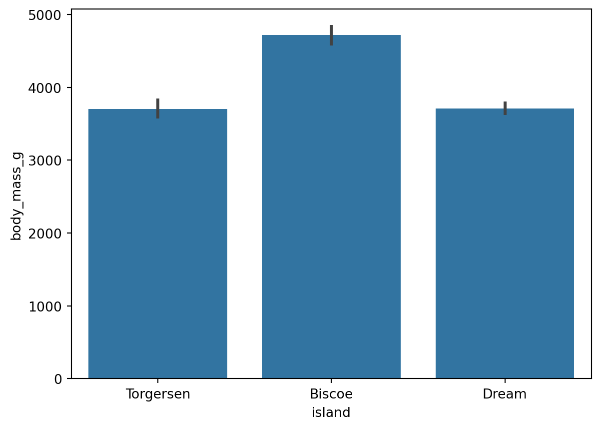
# estimator='sum':将柱高改为求和(默认为均值)
sns.barplot(data=df, x='island', y='body_mass_g', estimator='sum')
plt.show()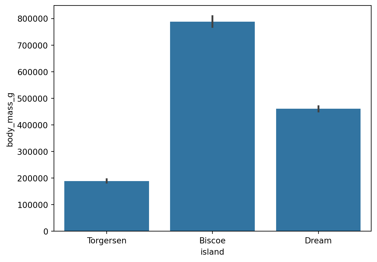
参考:sns.barplot() 函数的用法(estimator 参数)
sns.__version__ # 查看当前 Seaborn 版本(0.13 起默认单色,避免无意义的颜色区分)'0.13.2'# 验证:Biscoe 岛体质量均值即为柱状图对应的柱高
df.loc[df['island'] == 'Biscoe', 'body_mass_g'].mean()4716.017964071856# 计数图:自动统计每个类别的出现次数
sns.countplot(data=df, x='species')
plt.show()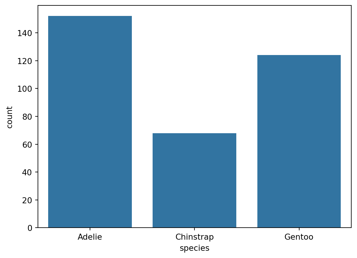
使用 hue 参数按类别分组,设置 errorbar=None 去除误差线。
# hue 按性别分组显示,errorbar=None 去除误差线
sns.barplot(data=df, x='island', y='body_mass_g', errorbar=None, hue='sex')
plt.show()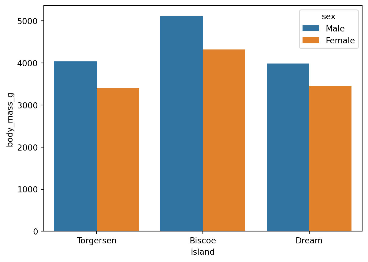
参考:sns.barplot() 函数的用法(errorbar 参数、hue 参数)
x 轴标签过长时,可用 plt.xticks() 旋转标签:
sns.barplot(data=df, x='island', y='body_mass_g', errorbar=None, hue='sex')

# 标签旋转 45°,ha='right' 使标签右端与刻度线对齐
plt.xticks(rotation=45, ha='right')
plt.show()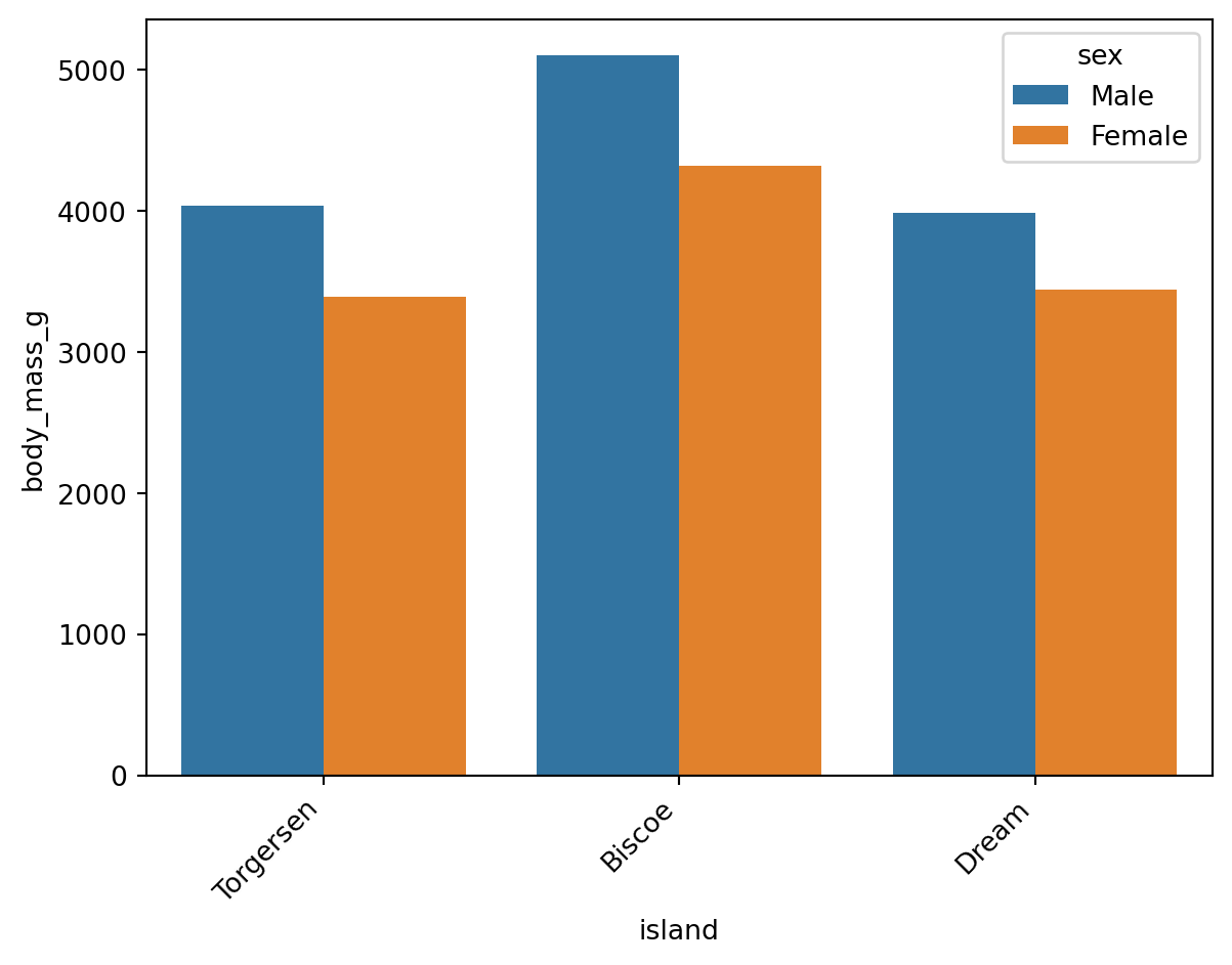
参考:plt.xticks() 函数用法(kwargs 栏目)
Wilke (2019, chap. 6.1) 建议:标签密集时,改为横向排版比旋转标签更易读:
# 交换 xy 轴:标签密集时横向排版更易读
sns.barplot(data=df, y='island', x='body_mass_g', errorbar=None, hue='sex')
plt.show()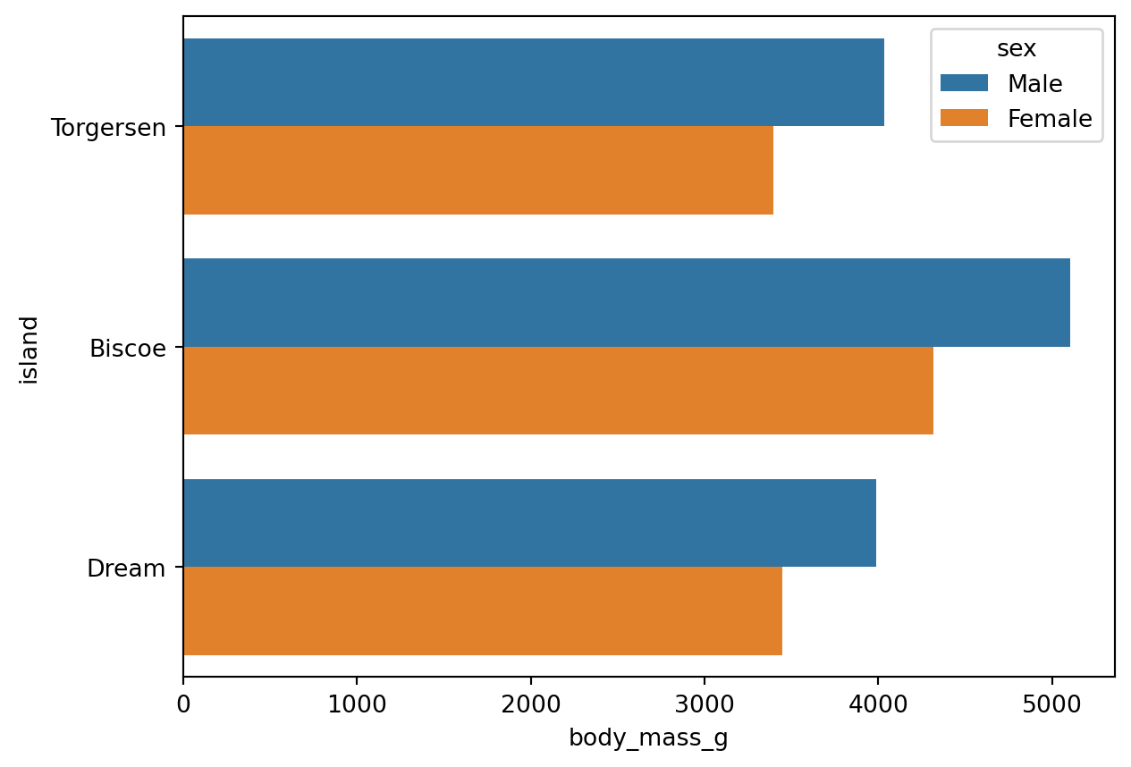
同样适用于 Count Plot:
sns.countplot(data=df, y='species', hue='sex')
plt.show()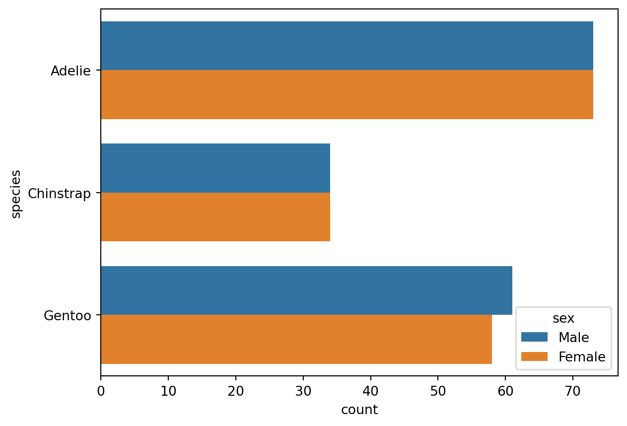
# 设置全局绘图主题(作用于后续所有 Seaborn 图表,可用 sns.reset_orig() 还原)
sns.set_theme(font_scale=1.2, style='darkgrid')
sns.set_theme() 设置全局绘图主题,作用于之后所有 Seaborn 图表。调用 sns.reset_orig() 可恢复默认主题。
# 定义一个图表对象 ax
ax = sns.barplot(
    data=df, x='body_mass_g', y='island',
    errorbar=None, hue='sex',
)

# 设置标题与轴标签
ax.set(title='Penguin', xlabel='Body Mass (g)', ylabel='Island')
plt.show()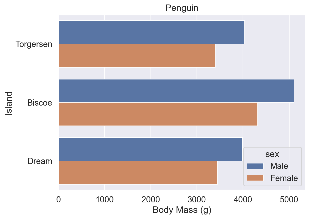
将 Seaborn 图表赋值给变量 ax 后,可调用 Matplotlib 方法进一步修改(类似将 DataFrame 赋值给 df 后再调用方法)。
注意:区分以下两者:
sns.set() / sns.set_theme():Seaborn 全局主题设置函数(两者等价,sns.set_theme() 为首选)。ax.set():Matplotlib 中针对特定图表对象的方法,用于设置标题、轴标签等。无论 errorbar=None 还是 errorbar=('ci',0),图例均可能遮挡图表,需用 sns.move_legend() 手动调整位置。
# errorbar=None:图例自动置于右侧
ax = sns.barplot(data=df, y='island', x='body_mass_g', errorbar=None, hue='sex')
ax.set(title='Penguin', xlabel='Body Mass (g)', ylabel='Island')
plt.show()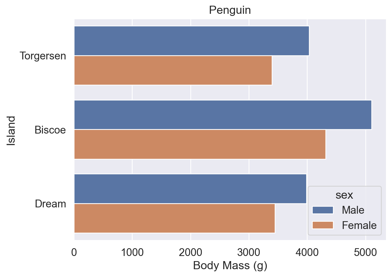
# errorbar=('ci', 0):图例自动避让误差线区域
ax = sns.barplot(
    data=df, y='island', x='body_mass_g',
    errorbar=('ci', 0), hue='sex',
)
ax.set(title='Penguin', xlabel='Body Mass (g)', ylabel='Island')
plt.show()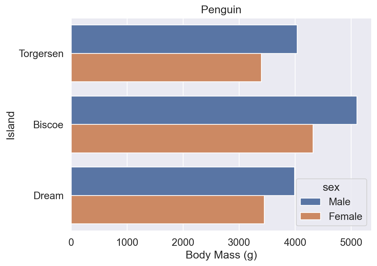
ax = sns.barplot(data=df, y='island', x='body_mass_g', errorbar=None, hue='sex')
ax.set(title='Penguin', xlabel='Body Mass (g)', ylabel='Island')

# bbox_to_anchor + loc 联用:将图例的 loc 参考点移至坐标 (0.5, -0.2)
sns.move_legend(ax, bbox_to_anchor=(0.5, -0.2), loc='upper center', ncols=2)
plt.show()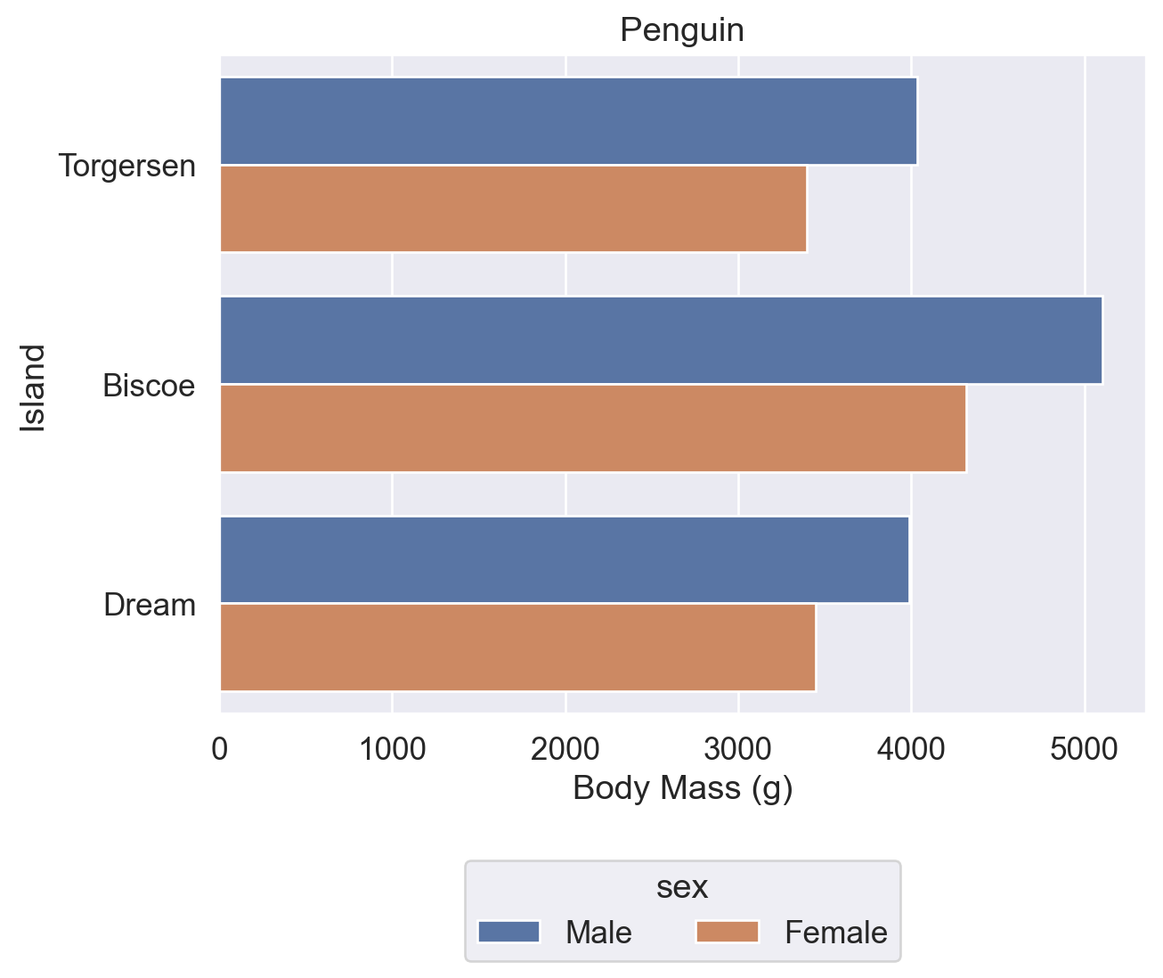
ax = sns.barplot(data=df, y='island', x='body_mass_g', errorbar=None, hue='sex')
ax.set(title='Penguin', xlabel='Body Mass (g)', ylabel='Island')
sns.move_legend(ax, loc='lower right')  # 仅设置 loc:图例移至图表右下角
plt.show()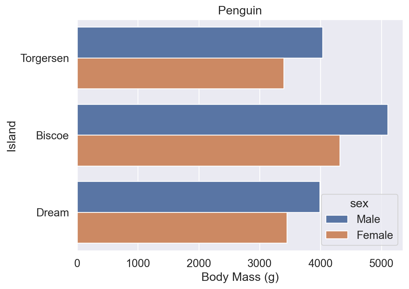
ax = sns.barplot(data=df, y='island', x='body_mass_g', errorbar=None, hue='sex')
ax.set(title='Penguin', xlabel='Body Mass (g)', ylabel='Island')

# 图例左上角置于图表 (1, 1) 处
sns.move_legend(ax, loc='upper left', bbox_to_anchor=(1, 1))
plt.show()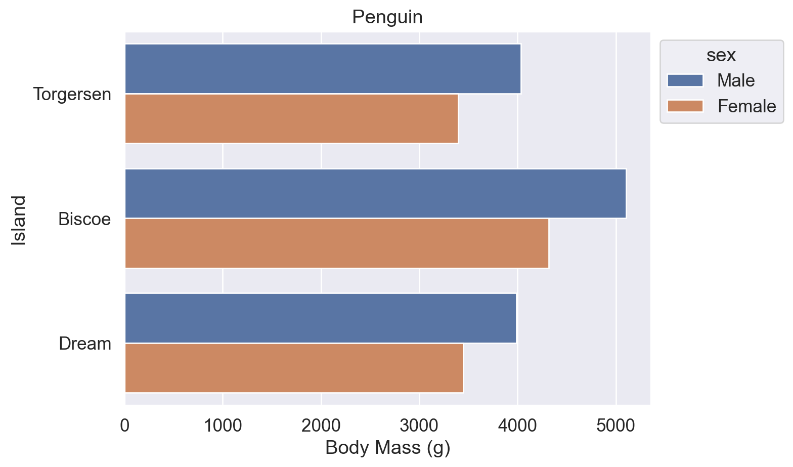
参考:
sns.move_legend() 用法(obj 参数、loc 参数)
matplotlib.axes.Axes.legend() 用法(loc、ncols、bbox_to_anchor 参数)
使用 palette 参数修改图表配色,可传入以下类型的值:
'deep'):'deep'、'muted'、'bright'、'pastel'、'dark'、'colorblind''viridis'、'plasma'、'coolwarm'、'Blues'、'Reds''hls'、'husl''ch:<args>',如 'ch:s=0.5,r=-0.5'(色盲友好,支持灰度打印)'light:<color>'、'dark:<color>''blend:<color1>,<color2>'['#FF5733', '#33FF57'])、RGB 元组、Matplotlib 颜色名称# 默认调色板
ax = sns.barplot(data=df, y='island', x='body_mass_g', errorbar=None, hue='sex')
ax.set(title='Penguin', xlabel='Body Mass (g)', ylabel='Island')
sns.move_legend(ax, bbox_to_anchor=(1, 1), loc='upper left')
plt.show()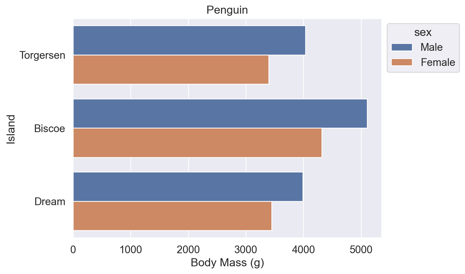
# palette='flare':使用 Seaborn 预设调色板
ax = sns.barplot(data=df, y='island', x='body_mass_g', errorbar=None, hue='sex', palette='flare')
ax.set(title='Penguin', xlabel='Body Mass (g)', ylabel='Island')
sns.move_legend(ax, bbox_to_anchor=(1, 1), loc='upper left')
plt.show()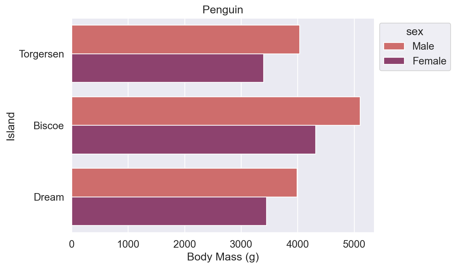
# palette 传入 Matplotlib 颜色名称列表
ax = sns.barplot(data=df, y='island', x='body_mass_g', errorbar=None, hue='sex', palette=['blue', 'orange'])
ax.set(title='Penguin', xlabel='Body Mass (g)', ylabel='Island')
sns.move_legend(ax, bbox_to_anchor=(1, 1), loc='upper left')
plt.show()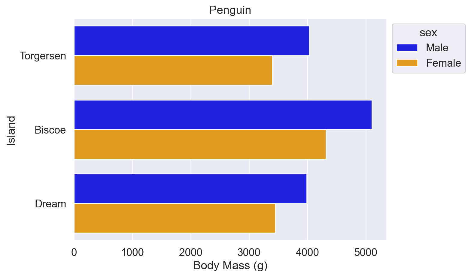
# palette 传入十六进制颜色代码列表
ax = sns.barplot(
    data=df, y='island', x='body_mass_g',
    errorbar=None, hue='sex', palette=['#a1c9f4', '#8de5a1'],
)
ax.set(title='Penguin', xlabel='Body Mass (g)', ylabel='Island')
sns.move_legend(ax, bbox_to_anchor=(1, 1), loc='upper left')
plt.show()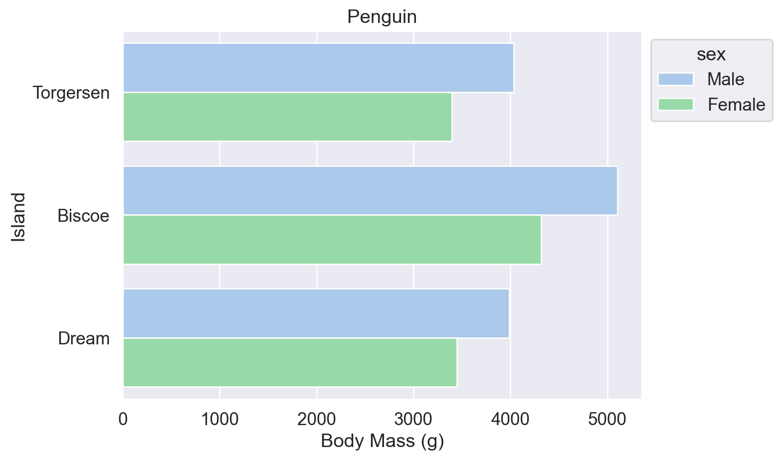
参考:
Seaborn sns.set_theme() 函数(palette 参数)
Seaborn sns.color_palette() 函数(预设调色盘名称表)
Matplotlib 预命名颜色一览
Matplotlib Colormap 一览
w3schools 颜色提取器
以下两种方式等效,可用于后续按总量排序柱状图。
法1:df.groupby().size()
# 按 island 分组后统计每组行数
df.groupby('island').size()
island
Biscoe 168
Dream 124
Torgersen 52
dtype: int64法2:df.value_counts()
# 统计 island 列中各值的出现次数
df.value_counts('island')
island
Biscoe 168
Dream 124
Torgersen 52
Name: count, dtype: int64柱状图的纵轴必须从 0 开始,以保证视觉比例与数据比例一致(Wilke (2019, chap.17) 的 Principle of Proportional Ink)。点线图无此限制,纵轴从数据范围起始,且 data-ink ratio 更高(干扰信息更少)。
当 x 轴为 nominal data(如岛屿名称)时,各点之间无需连线。
# linestyle='none':x 轴为离散类别时不连线;点上下的线段为误差线
sns.pointplot(data=df, x='island', y='body_mass_g', hue='sex', linestyle='none')
plt.show()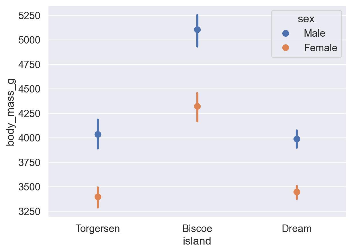
柱状图的 x 轴为离散类别(nominal/ordinal data);直方图的 x 轴为连续数值区间(ratio data)。
sns.histplot(data=df, x='flipper_length_mm')
plt.show()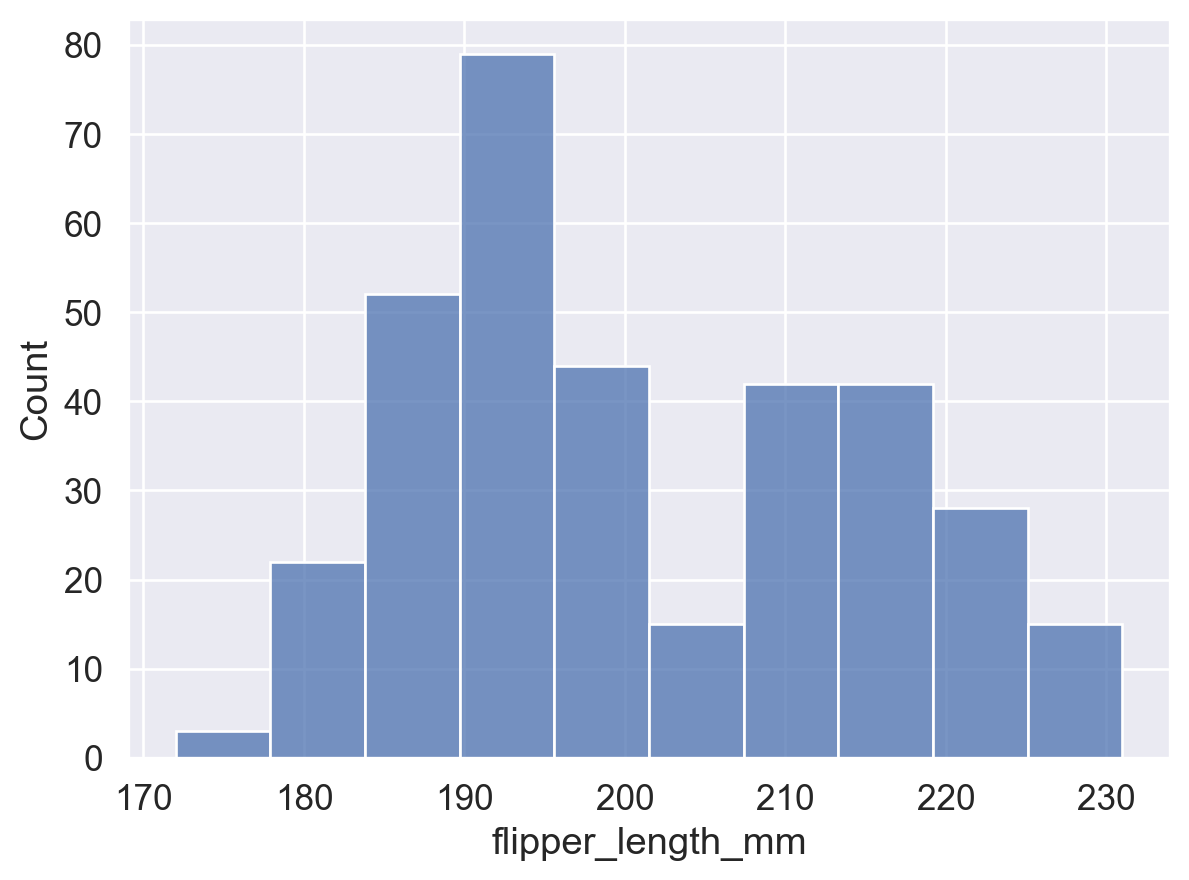
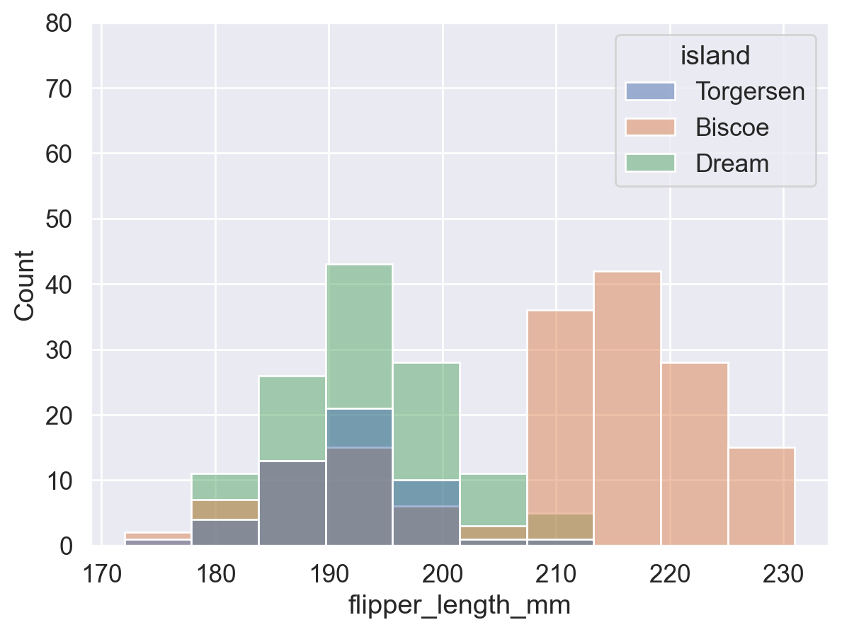
# hue 分组:各岛企鹅分别绘图后叠加显示
sns.histplot(data=df, x='flipper_length_mm', hue='island')
plt.show()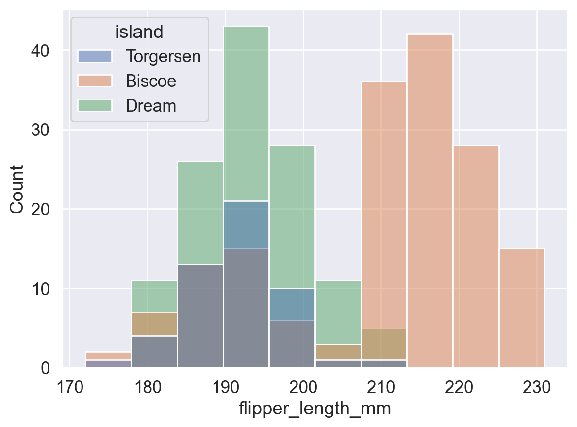
# 统一 y 轴范围,对比有无 hue 分组的差异
sns.histplot(data=df, x='flipper_length_mm')
plt.show()

sns.histplot(data=df, x='flipper_length_mm', hue='island')
plt.ylim(0, 80)
plt.show()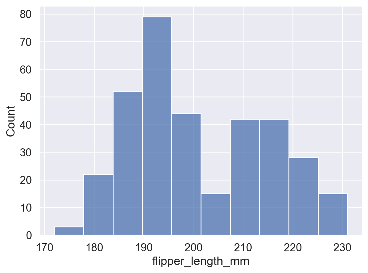
sns.histplot(
    data=df, x='flipper_length_mm',
    hue='island',
    stat='density',     # 各 bin 面积之和为 1(概率密度)
    common_norm=False   # 各组独立归一化 (每组面积和为1, 若 True 则所有面积和为1)
)
plt.show()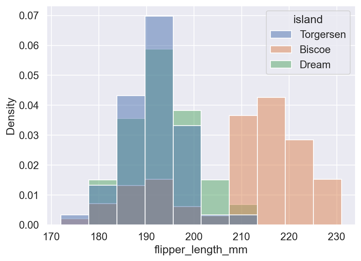
控制直方图的统计方式,可选值:
'count':bin 高度 = 该 bin 内的数据点数量(频数)。'frequency':bin 高度 = 频数 / bin 宽度(单位宽度内的频数,适用于 bin 宽度不统一的情况)。'probability' / 'proportion':bin 高度 = 频数 / 总数,所有 bin 高度之和为 1。'percent':bin 高度 = (频数 / 总数) × 100,所有 bin 高度之和为 100。'density':bin 高度 = 频率 / 组距,所有 bin 面积之和为 1(频率分布直方图)。当 bin 宽度趋近于 0 时,即得到平滑密度曲线。# stat='count':柱高 = bin 内数据点数量
ax = sns.histplot(data=df, x='flipper_length_mm', stat='count')
# 遍历每个柱子(patch),获取高度并在柱顶显示数值标签
for p in ax.patches:
# 获取柱子高度(即区间内的数据点频数)
height = p.get_height()
# 添加文字
ax.text(
p.get_x() + p.get_width() / 2, # x(文字横坐标): 柱子中心位置
height, # y(文字纵坐标): 柱子高度
int(height), # str(文字内容): 显示整数频数
ha='center', va='bottom', # horizontal/vertical anchor (水平/垂直对齐方式)
)
plt.show()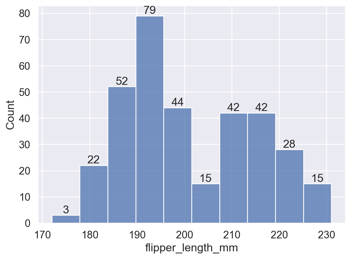
# stat='frequency':柱高 = 频数 / bin 宽度
ax = sns.histplot(data=df, x='flipper_length_mm', stat='frequency')
for p in ax.patches:
    height = p.get_height()
    ax.text(
        p.get_x() + p.get_width() / 2,
        height, int(height),
        ha='center', va='bottom',
    )
plt.show()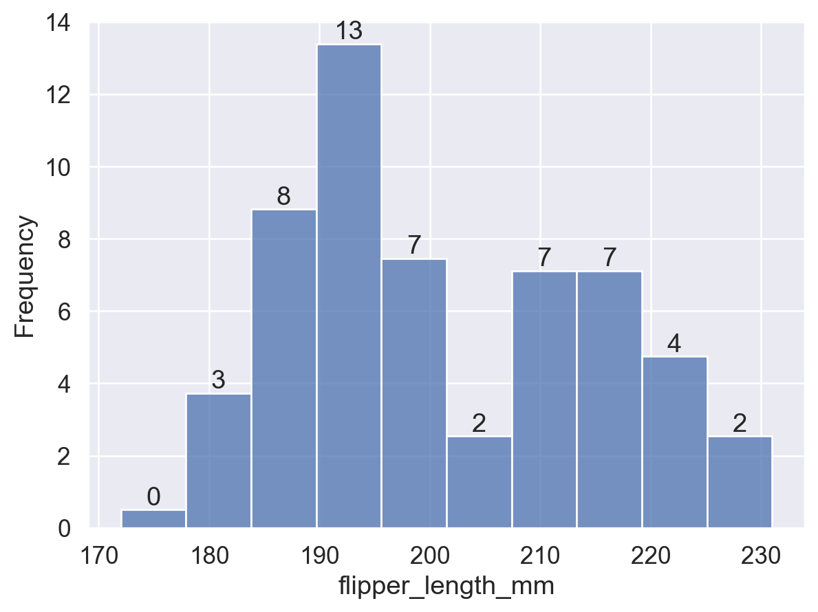
# stat='probability':柱高 = 频数 / 总数,所有柱高之和为 1
ax = sns.histplot(data=df, x='flipper_length_mm', stat='probability')
for p in ax.patches:
    height = p.get_height()
    ax.text(
        p.get_x() + p.get_width() / 2,
        height, f'{height:.2f}', # 保留两位小数
        ha='center', va='bottom',
    )
plt.show()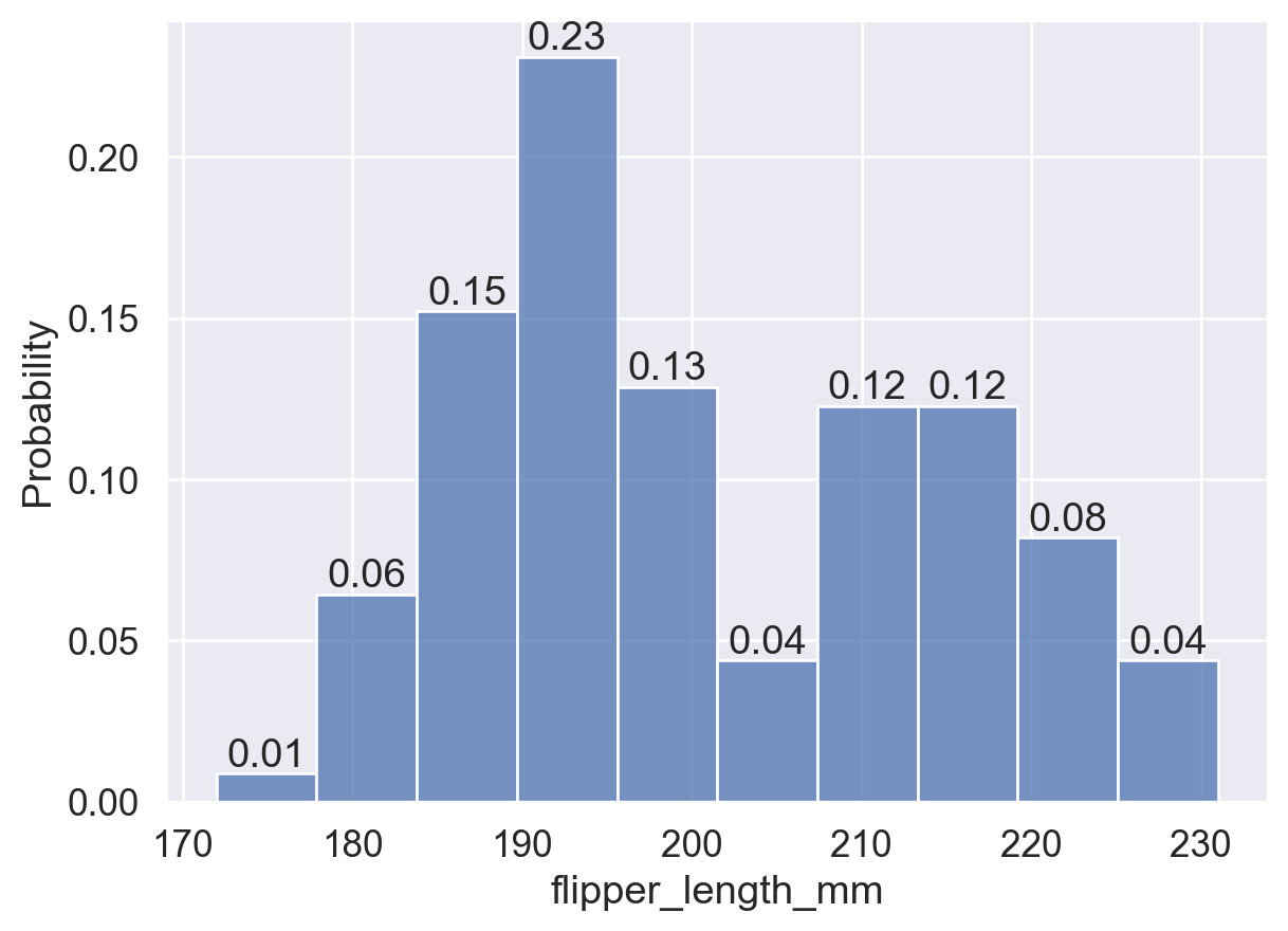
# stat='percent':柱高 = (频数 / 总数) × 100,所有柱高之和为 100
ax = sns.histplot(data=df, x='flipper_length_mm', stat='percent')
for p in ax.patches:
    height = p.get_height()
    ax.text(
        p.get_x() + p.get_width() / 2,
        height, int(height),
        ha='center', va='bottom',
    )
plt.show()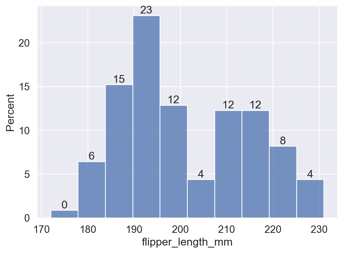
# stat='density':柱高 = 频率 / 组距,所有 bin 面积之和为 1
ax = sns.histplot(data=df, x='flipper_length_mm', stat='density')
for p in ax.patches:
    height = p.get_height()
    ax.text(
        p.get_x() + p.get_width() / 2,
        height, f'{height:.3f}',
        ha='center', va='bottom',
    )
plt.show()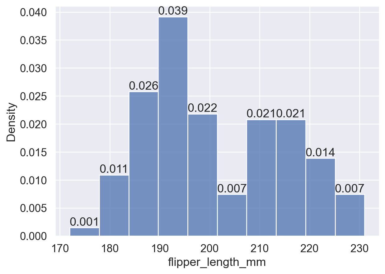
布尔值,仅在 stat 为 'probability'、'proportion'、'percent' 或 'density' 时生效,默认为 True:
common_norm=True:基于整个数据集归一化,不同组间的 bin 高度可直接比较。common_norm=False:各子组独立归一化,bin 高度仅在组内有意义。sns.histplot(
data=df, x='flipper_length_mm', hue='island',
stat='density', common_norm=True, # 整体归一化:所有组的 bin 面积总和为 1
)
plt.show()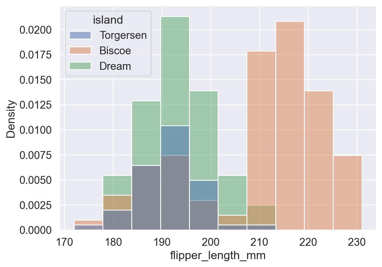
sns.histplot(
    data=df, x='flipper_length_mm', hue='island',
    stat='density', common_norm=False, # 各组独立归一化: 每组 bin 面积之和分别为 1
)
plt.show()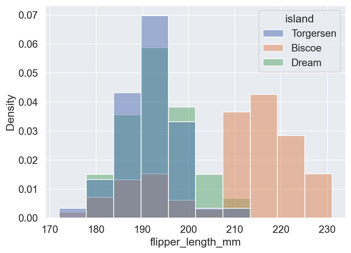
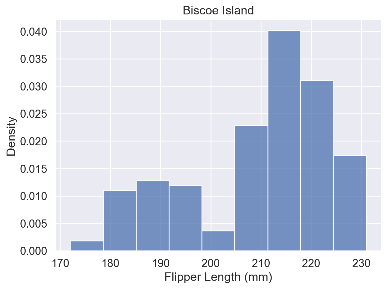
分组重叠不清晰时,可用 data=df[df['列']==值] 筛选数据,为各组分别绘图:
# 分岛绘图,避免分组叠加,逐一观察各岛分布
ax = sns.histplot(
    data=df[df['island'] == 'Torgersen'],
    x='flipper_length_mm', stat='density'
)
ax.set(title='Torgersen Island', xlabel='Flipper Length (mm)')
plt.show()

ax = sns.histplot(
    data=df[df['island'] == 'Biscoe'],
    x='flipper_length_mm', stat='density'
)
ax.set(title='Biscoe Island', xlabel='Flipper Length (mm)')
plt.show()

ax = sns.histplot(
    data=df[df['island'] == 'Dream'],
    x='flipper_length_mm', stat='density'
)
ax.set(title='Dream Island', xlabel='Flipper Length (mm)')
plt.show()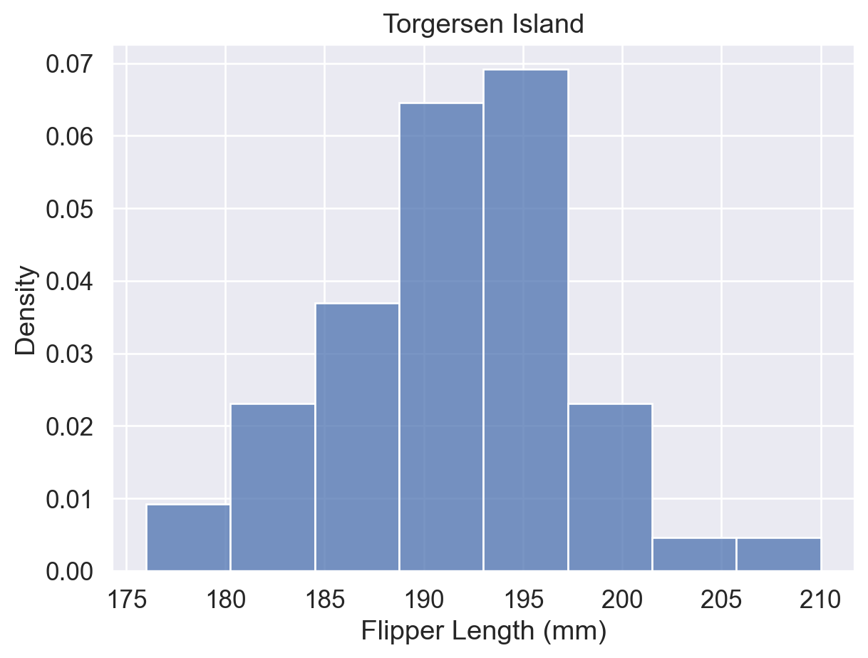
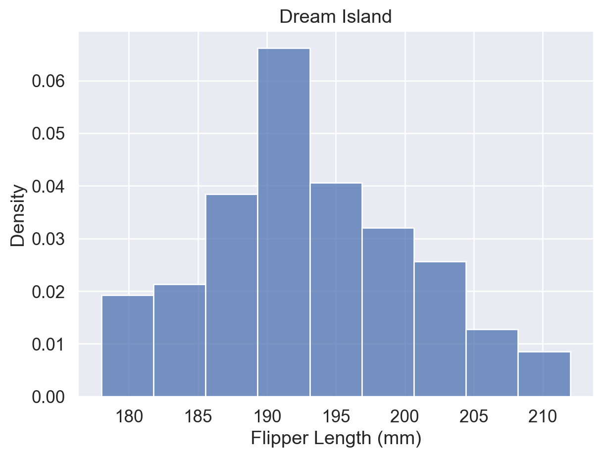
参考:sns.histplot() 函数用法(hue、stat、common_norm 参数)
箱线图(boxplot)通过五个关键值概括数据分布:Min、Q1、Q2(中位数)、Q3、Max,并标记超出须范围的异常值。
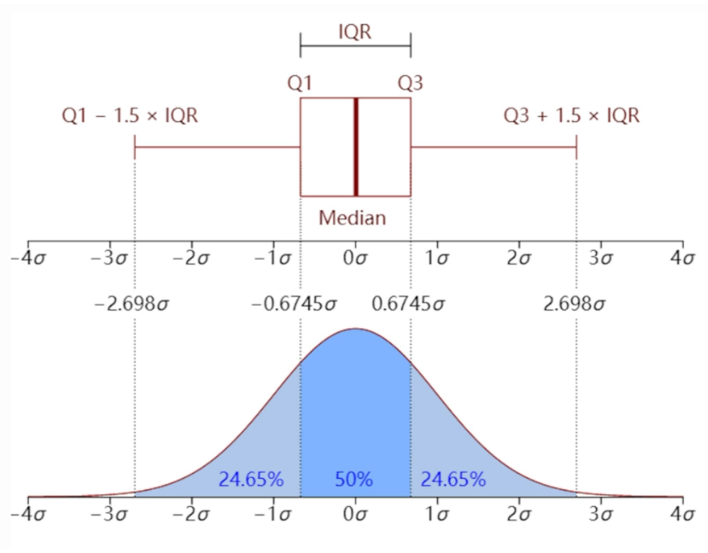
箱线图 vs. 直方图
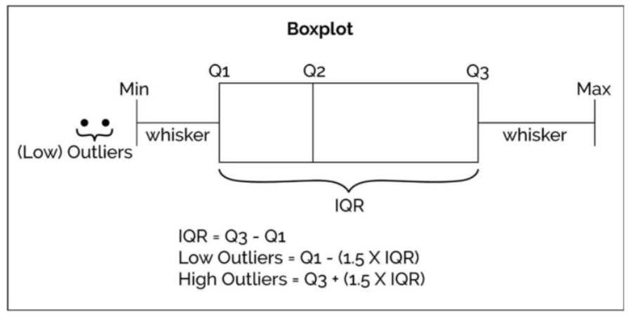
箱线图适合快速识别分布概况与异常值;直方图适合查看具体区间内的频率分布。
sns.boxplot(data=df, x='flipper_length_mm', y='island', hue='sex')
plt.show()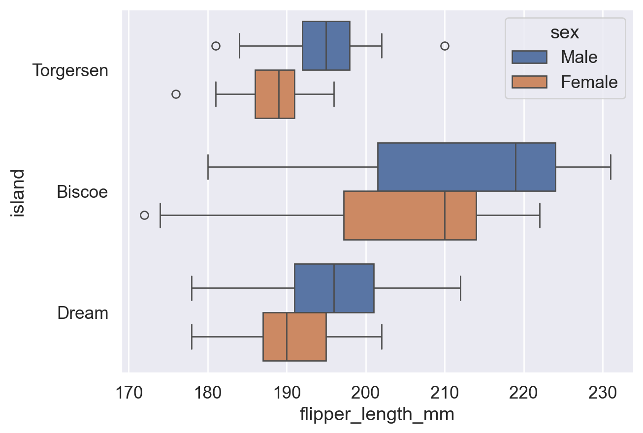
sns.boxplot(
    data=df, x='flipper_length_mm', y='island', hue='sex',
    fliersize=8,  # fliersize: 异常点大小(默认 5)
)
plt.show()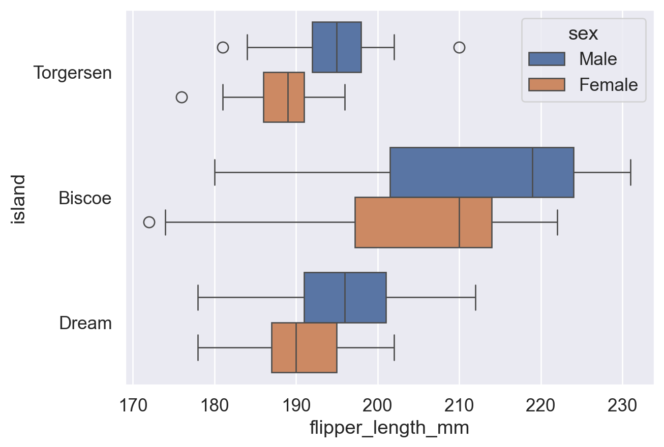
sns.boxplot(
    data=df, x='flipper_length_mm', y='island', hue='sex', fliersize=8,
    whis=2,  # whisker:须延伸至 Q1/Q3 ± 2×IQR(默认 1.5),更大值减少异常点
)
plt.show()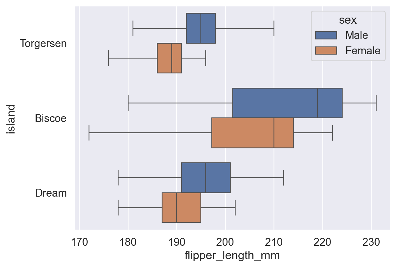
参考:sns.boxplot() 函数用法(fliersize、whis 参数)
小提琴图结合了箱线图(中位数、分位数)与密度曲线(平滑分布)的特点。数据量较少时,平滑曲线可能失真,建议改用直方图或箱线图。
sns.violinplot(data=df, y='island', x='flipper_length_mm', hue='sex')
plt.show()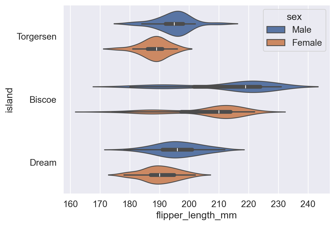
# split=True: 将同类别的两组合并为同一小提琴,便于对比分布形态
sns.violinplot(
    data=df, y='island', x='flipper_length_mm', hue='sex',
    split=True, # 将两个 hue 不同的组分布合并为同一小提琴,便于对比分布形态
)
plt.show()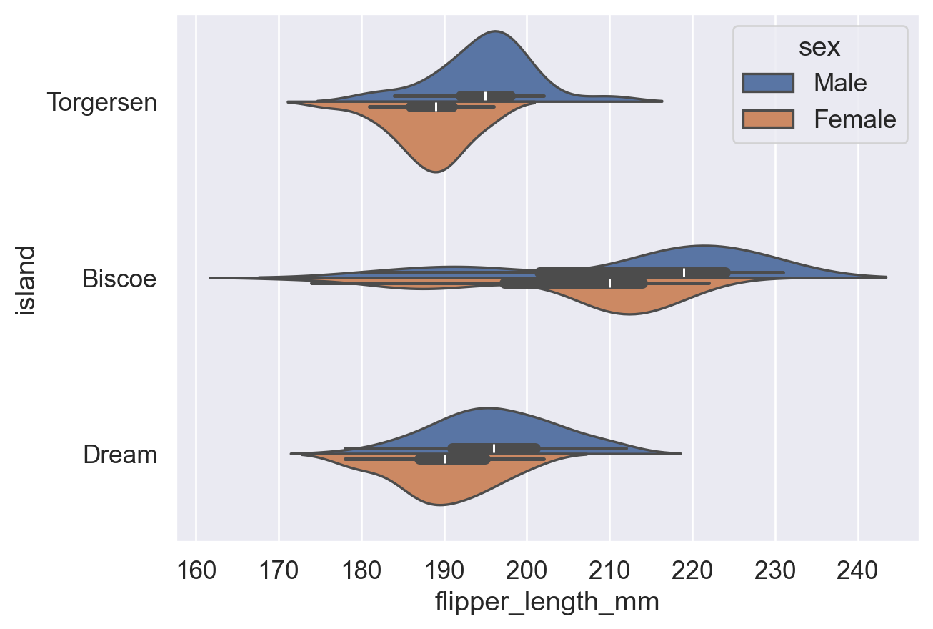
参考:sns.violinplot() 函数用法(split 参数)
条带图 (strip plot) 绘制所有数据点 (每点圆点是一个数据点) 并随机抖动 (同一数值下的点随机沿轴向抖动, 为了避免数据点重叠), 展示数据分布情况;蜂群图 (swarm plot) 自动排列重叠的数据点, 可读性更高。
注意:两者均展示单变量分布(某数据在各区间的密度),不同于展示两变量相关趋势的 scatter plot。
| 对比维度 | strip plot(散点条带图) | swarm plot(蜂群图) |
|---|---|---|
| 基本概念 | 将数据点沿分类轴随机抖动(jitter)以避免重叠 | 通过算法精确排列点,避免重叠并展示分布 |
| 点的排列方式 | 随机抖动,可能仍有重叠 | 非随机,基于密度自动调整位置,完全避免重叠 |
| 可读性 | 数据量小时较清晰,数据量大时容易重叠 | 在中小规模数据中更清晰展示分布形状 |
| 计算复杂度 | 较低,绘制速度快 | 较高,数据量大时绘制较慢 |
| 适用场景 | 快速可视化、小数据集、对精确分布要求不高 | 展示数据分布细节、中等规模数据 |
| 分布表现能力 | 一般,难以体现真实密度 | 较强,可直观体现数据密度 |
| 参数控制 | 可通过 jitter 控制抖动程度 |
无需 jitter,由算法自动调整 |
| 示例函数 | sns.stripplot() |
sns.swarmplot() |
sns.stripplot(data=df, x='flipper_length_mm', y='island', hue='sex')
plt.show()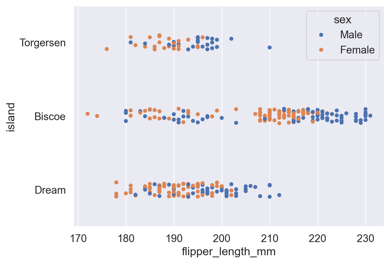
sns.swarmplot(data=df, x='flipper_length_mm', y='island', hue='sex')
plt.show()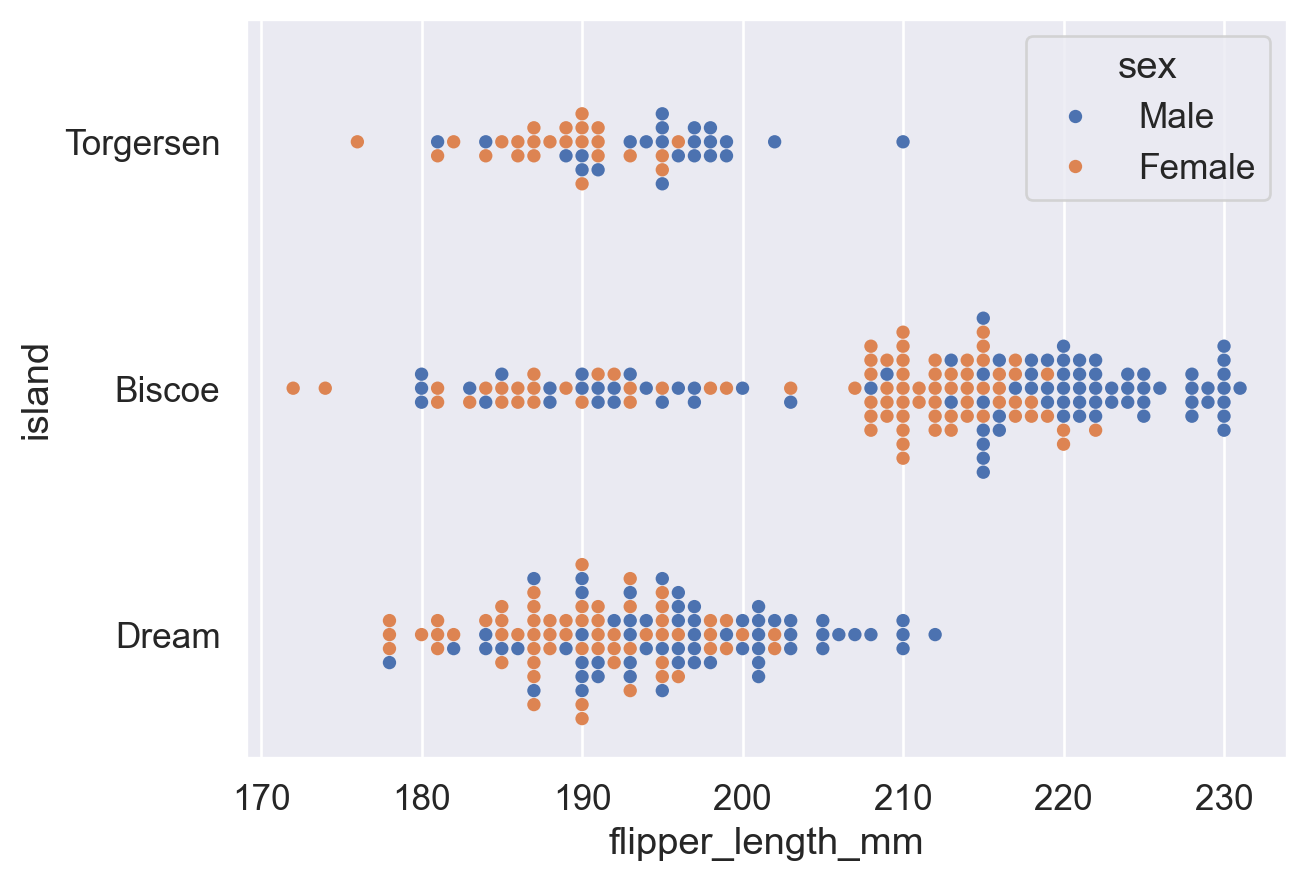
总体链接:
Python3 教程文档 (中文) (查看内置函数用法等)
Pandas库 教程文档 (DataFrame)
Matplotlib库 教程文档 (plt)
Seaborn库 教程文档 (barplot)
sns.barplot()函数(用 Seaborn 绘制 柱状图)
sns.countplot()函数 (用 Seaborn 绘制 计数图)修改图表主题风格:
plt.xticks()函数 ( kwargs (keyword argument) 栏目中写了如何旋转刻度标签)
sns.set()函数 (同sns.set_theme()函数)
sns.set_theme()函数 (设置 Seaborn 绘图的全局主题风格)
ax.set()方法 (Matplotlib 中 对于特定图表 ax 设置标题、轴标签等元素的方法)修改图例:
sns.move_legend()函数 (Seaborn 中 移动图例的函数)(查看 obj参数 和 loc参数 的用法)
matplotlib.axes.Axes.legend()函数 (Matplotlib 中 设置图例的函数,其指令也适用于sns.move_legend())(查看 loc参数 ,ncols参数 和 bbox_to_anchor参数 的用法)修改图表颜色:
Seabornsns.color_palette()函数 (查看 palette参数 预设调色盘名称表)
Matplotlib 预命名颜色一览
Matplotlib Colormap 一览
Matplotlib Colormap 使用介绍
w3schools 颜色提取器 (查看任意颜色的十六进制代码)其他图表:
sns.pointplot()函数用法 (点线图画法)
sns.histplot()函数用法 (频率分布直方图画法)(查看 hue参数 ,stat参数 和 common_norm参数 )
sns.boxplot()函数用法 (箱线图画法) (查看 fliersize参数 和 whis参数 )
sns.violinplot()函数用法 (小提琴图画法)
sns.stripplot()函数 (分布散点图画法)
sns.swarmplot()函数 (分簇分布散点图画法)教材书 Fundamentals of Data Visualization (Wilke, 2019) :
6.1 Bar Plot (旋转的文字刻度不方便阅读,应当横过来排版)
17. The Principle of Proportional Ink (比例标记的原则:图形大小比例应当和数据真实的比例一样。e.g. 柱状图的柱子应当从 0 开始)