环境与版本
python==3.12
pandas==2.2.2
matplotlib==3.9.x
seaborn==0.13.2python==3.12
pandas==2.2.2
matplotlib==3.9.x
seaborn==0.13.2本项目使用一份关于西班牙加泰罗尼亚公投的 Twitter 推文数据集,属性包括每条推文的基本信息及由不同词典检测到的情感词计数 (Jiménez-Zafra 等, 2021)(属性详细说明见附录一)。本文通过条形图展示各词典在推文情感检测上的表现差异,并以直方图按情感类别呈现所有推文的作者受欢迎度分布。
# 导入库
import pandas as pd   # 数据处理
import matplotlib.pyplot as plt   # 绘图
import seaborn as sns   # 绘图

# 读取 CSV 文件
df = pd.read_csv(
    '../../../src/data/Catalan_Referendum_Twitter_corpus.csv',
    encoding = 'latin',  # 非 UTF-8 编码
    delimiter = ';',
)

# 预览数据
df.head()| lang | retweet_count | favorite_count | is_quote_status | num_hashtags | num_urls | num_mentions | interval_time | positive_words_iSOL | negative_words_iSOL | positive_words_NRC | negative_words_NRC | positive_words_mlSenticon | negative_words_mlSenticon | verified_user | followers_count_user | friends_count_user | listed_count_user | favourites_count_user | statuses_count_user | |
|---|---|---|---|---|---|---|---|---|---|---|---|---|---|---|---|---|---|---|---|---|
| 0 | es | 0 | 0.0 | False | 2.0 | 0 | 0.0 | tarde-noche | 0.0 | 0.0 | 0.0 | 1.0 | 0 | 0.0 | False | 459.0 | 741.0 | 4.0 | 140.0 | 2880.0 |
| 1 | es | 0 | 1.0 | False | 1.0 | 1 | 0.0 | tarde-noche | 0.0 | 0.0 | 0.0 | 1.0 | 0 | 0.0 | False | 7995.0 | 996.0 | 194.0 | 10335.0 | 23859.0 |
| 2 | es | 3 | 5.0 | False | 1.0 | 1 | 0.0 | tarde-noche | 1.0 | 1.0 | 0.0 | 0.0 | 1 | 0.0 | True | 151704.0 | 2201.0 | 250.0 | 10321.0 | 229298.0 |
| 3 | es | 0 | 1.0 | False | 1.0 | 0 | 0.0 | tarde-noche | 0.0 | 0.0 | 0.0 | 0.0 | 0 | 0.0 | False | 2199.0 | 1641.0 | 7.0 | 2386.0 | 49363.0 |
| 4 | es | 0 | 0.0 | False | 2.0 | 1 | 0.0 | tarde-noche | 0.0 | 2.0 | 0.0 | 2.0 | 0 | 1.0 | False | 1319.0 | 170.0 | 22.0 | 962.0 | 2410.0 |
## 删除缺失值(见附录二)
df = df.dropna()

## 抽取 1000 行样本并重置索引
df = df.sample(1000, random_state = 32).reset_index(drop = True)

## 重命名列以提升可读性
# 1) 统一 favorite/favourites 拼写
# 2) 明确 statuses_count_user 的含义
df = df.rename(
    columns = {
        'favorite_count':'like_count',
        'favourites_count_user':'likes_count_user',
        'statuses_count_user':'tweets_count_user',
    }
)# 检查属性数据类型
df.info()<class 'pandas.core.frame.DataFrame'>
RangeIndex: 1000 entries, 0 to 999
Data columns (total 20 columns):
# Column Non-Null Count Dtype
--- ------ -------------- -----
0 lang 1000 non-null object
1 retweet_count 1000 non-null object
2 like_count 1000 non-null float64
3 is_quote_status 1000 non-null object
4 num_hashtags 1000 non-null float64
5 num_urls 1000 non-null object
6 num_mentions 1000 non-null float64
7 interval_time 1000 non-null object
8 positive_words_iSOL 1000 non-null float64
9 negative_words_iSOL 1000 non-null float64
10 positive_words_NRC 1000 non-null float64
11 negative_words_NRC 1000 non-null float64
12 positive_words_mlSenticon 1000 non-null object
13 negative_words_mlSenticon 1000 non-null float64
14 verified_user 1000 non-null object
15 followers_count_user 1000 non-null float64
16 friends_count_user 1000 non-null float64
17 listed_count_user 1000 non-null float64
18 likes_count_user 1000 non-null float64
19 tweets_count_user 1000 non-null float64
dtypes: float64(13), object(7)
memory usage: 156.4+ KB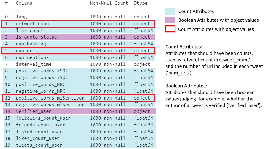
## 检查 3 个 object 类型计数属性的数据类型
print(df[['retweet_count', 'num_urls', 'positive_words_mlSenticon']].dtypes)

print("")

## 确认所有值都是数字字符串(可安全使用 .astype() 转换)
print(
    df['retweet_count'].str.isnumeric().all(),
    df['num_urls'].str.isnumeric().all(),
    df['positive_words_mlSenticon'].str.isnumeric().all()
)

## 将所有计数属性转换为整数
# object 转 int
df[[
    'retweet_count', 'num_urls', 'positive_words_mlSenticon',
]] = df[[
    'retweet_count', 'num_urls', 'positive_words_mlSenticon',
]].astype(int)

# float 转 int
float_cols = df.select_dtypes(include='float').columns  # 所有 float 列
df[float_cols] = df[float_cols].astype(int)
retweet_count object
num_urls object
positive_words_mlSenticon object
dtype: object
True True True# 确认布尔列只包含 'True'/'False' 字符串
print(df['is_quote_status'].unique())
print(df['verified_user'].unique())
# 将字符串布尔列转换为 bool 类型
df['is_quote_status']=df['is_quote_status'].map({'True':True, 'False':False})
df['verified_user']=df['verified_user'].map({'True':True, 'False':False})['False' 'True']
['False' 'True']## 将情感词计数列转换为长格式,便于可视化
# value_vars:所有情感计数列(各词典的正面/负面词计数)
# var_name:存储原始列名(包含情感类别和来源信息)
# value_name:存储对应计数
df_melted = df.melt(
value_vars = [
'positive_words_iSOL','negative_words_iSOL',
'positive_words_NRC','negative_words_NRC',
'positive_words_mlSenticon','negative_words_mlSenticon',
],
var_name = 'sentiment_and_source',
value_name = 'count',
)
df_melted.head() # 初始长格式结果,尚未进一步处理| sentiment_and_source | count | |
|---|---|---|
| 0 | positive_words_iSOL | 0 |
| 1 | positive_words_iSOL | 0 |
| 2 | positive_words_iSOL | 0 |
| 3 | positive_words_iSOL | 0 |
| 4 | positive_words_iSOL | 0 |
## 添加情感类别列(正面/负面)

# 以下变量分别返回布尔序列,用于检查
# sentiment_and_source 是否包含指定关键词
is_positive = df_melted['sentiment_and_source'].str.contains('positive')
is_negative = df_melted['sentiment_and_source'].str.contains('negative')

# 按索引将'正面'/'负面'赋值给新的情感类别列
df_melted.loc[df_melted[is_positive].index,'sentiment'] = '正面'
df_melted.loc[df_melted[is_negative].index,'sentiment'] = '负面'

## 添加来源列(词典名称)
is_iSOL = df_melted['sentiment_and_source'].str.contains('iSOL')
is_NRC = df_melted['sentiment_and_source'].str.contains('NRC')
is_mlSenticon = df_melted['sentiment_and_source'].str.contains('mlSenticon')
df_melted.loc[df_melted[is_iSOL].index,'source'] = 'iSOL'
df_melted.loc[df_melted[is_NRC].index,'source'] = 'NRC'
df_melted.loc[df_melted[is_mlSenticon].index,'source'] = 'mlSenticon'

## 删除已经冗余的 sentiment_and_source 列
df_melted = df_melted.drop(columns = 'sentiment_and_source')
df_melted.head()  # 情感类别和来源现已拆分为独立列

##############################################################################
## 设置 seaborn 主题并绘制条形图

sns.set_theme(
    font_scale = 1.2,
    style = 'whitegrid',
    rc = {
        'font.family': [
            'Arial Unicode MS', 'Heiti TC', 'Arial',
        ],
        'axes.unicode_minus': False,
    },
)

sns.barplot(
    data = df_melted, x = 'source', y = 'count', hue = 'sentiment',
    # 调色板:salmon(暖色)表示正面,royalblue(冷色)表示负面
    palette = ['salmon', 'royalblue'], errorbar = None,
)
plt.title('加泰罗尼亚公投的网络情感')
plt.ylim(0, 0.7)  # 设置 y 轴范围
plt.xlabel('情感分析词典')
plt.ylabel('平均情感词计数')
plt.legend(title = '情感类别')
plt.show()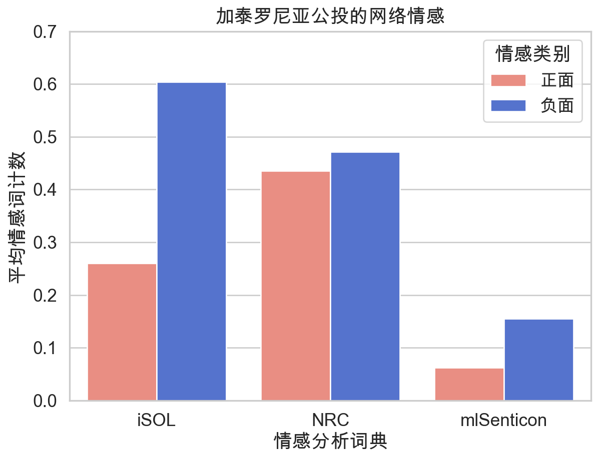
图 2 展示了所选加泰罗尼亚公投相关推文中,由三种情感分析词典(iSOL、NRC、mlSenticon)检测到的情感词平均计数,并按正面与负面情感分色呈现——暖红色”salmon”对应正面情感,冷蓝色”royalblue”对应负面情感,两者均为 Matplotlib 预定义颜色 (Matplotlib Development Team, 不详)。这两种颜色饱和度与亮度适中,有效避免视觉疲劳 (Wilke, 2019, chap. 19.1)。此外,颜色与情感的对应关系符合直觉,因为颜色的冷暖倾向通常与其所代表的情感相对应 (Hanada, 2018),从而提升了图表的”数据-墨水比” (Wilke, 2019, chap. 23)。
总体而言,负面情感词的数量始终多于正面情感词,反映了网络公众对加泰罗尼亚公投的总体负面态度。
从各词典的表现来看,NRC 在判断话语情感倾向方面可能最为均衡;而 mlSenticon 在本项目中的效果相对较弱,其正负情感的计数均为三者中最低。
以下公式用于计算推文作者的受欢迎度 (Riquelme & González-Cantergiani, 2016, pp. 6, 11):
\[Popularity(i) = 1 - e^{-λ·Fi} \]
受欢迎度表示用户的知名程度,其中 e 为自然对数的底数,λ 为常数。引入受欢迎度旨在创建一个在直方图中分布合理的比率型属性,因为原始比率属性(如粉丝数)过于分散,难以直观呈现。
## 定义受欢迎度计算函数
# F1:作者粉丝数;e ≈ 2.718,λ = 0.001
def calc_popularity(F1):
    result = 1 - 2.718 ** (-0.001*F1)
    return result

## 添加受欢迎度列
# 对 followers_count_user 逐行应用 calc_popularity
df['popularity'] = df['followers_count_user'].apply(calc_popularity)

## 定义总体情感判断函数(基于 iSOL 词典)
def determ_sentiment(row):
    if row['positive_words_iSOL'] > row['negative_words_iSOL']:
        return '正面'
    elif row['positive_words_iSOL'] < row['negative_words_iSOL']:
        return '负面'
    else:
        return '中立'

## 添加总体情感列
# axis=1:逐行应用函数
df['overall_sentiment'] = df.apply(determ_sentiment, axis=1)

## 绘制作者受欢迎度分布直方图
ax = sns.histplot(
    data = df, x = 'popularity',
    hue = 'overall_sentiment',
    hue_order = ['中立', '正面', '负面'],
    # 调色板:颜色与情感含义保持直观对应
    palette = ['lightgray', 'salmon', 'royalblue'],
    multiple = 'stack',  # 堆叠分组
    alpha = 0.9  # 透明度
)

# 更新图例标题(见附录三)
ax.get_legend().set_title('总体情感')
plt.title('作者受欢迎度分布直方图')
plt.xlabel('作者受欢迎度')
plt.ylabel('推文数量')
plt.ylim((0, 300))  # 设置 y 轴范围
plt.show()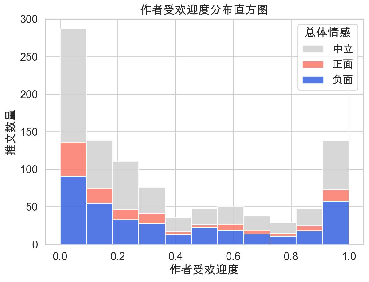
图 3 展示了推文按情感分组后的作者受欢迎度分布。总体而言,绝大多数参与者处于最低受欢迎度水平,随着作者受欢迎度的提升,推文数量逐渐减少,直至受欢迎度达到最高水平。此外,大多数推文为中立,而负面推文的数量多于正面推文。
这两张图仅分析了数据集中有限数量的属性,仍有改进空间。在数据类型处理完成后,其他属性同样可用于可视化。例如,转发数和点赞数等基本信息属性可用于估算每条推文的互动程度,并以直方图加以呈现。
本项目通过条形图分析了网络公众对加泰罗尼亚公投的总体态度,并比较了三种词典的表现。结果显示公众态度总体偏向负面,而 NRC 词典表现最为均衡。此外,受欢迎度较低的用户贡献了最多推文,这一结论通过按推文情感倾向分组的用户受欢迎度分布直方图得到呈现。
以下为原始数据集的整体介绍及数据集提供者对各属性的描述。
本语料库共包含 46,962 条与加泰罗尼亚公投相关的推文。加泰罗尼亚公投是西班牙一场极具争议的独立公投,由加泰罗尼亚地区政府发起,后经西班牙政府申请,被西班牙宪法法院宣布中止。所有推文均于 2017 年 10 月 1 日以话题标签 #CatalanReferendum 或 #ReferendumCatalan 下载。2017 年 10 月 31 日,我们进一步收集了这些推文的特征,以分析其传播性。语料库中的每条记录由我们用于病毒式传播分析的推文特征构成。
| 属性 | 说明 |
|---|---|
lang |
推文语言 |
retweet_count |
该推文被转发的总次数 |
favourite_count(重命名为 like_count) |
该推文被收藏的总次数 |
is_quote_status |
该推文是否引用了其他推文 |
num_hashtags |
推文中话题标签的总数 |
num_urls |
推文中 URL 的总数 |
num_mentions |
推文中提及用户的总数 |
interval_time |
推文发布的时间段(早晨 06:00–12:00、下午 12:00–18:00、晚上 18:00–00:00 或深夜 00:00–06:00) |
| 属性 | 说明 |
|---|---|
positive_words_iSOL |
使用 iSOL 词典检测到的推文正面词总数 |
negative_words_iSOL |
使用 iSOL 词典检测到的推文负面词总数 |
positive_words_NRC |
使用 NRC 词典检测到的推文正面词总数 |
negative_words_NRC |
使用 NRC 词典检测到的推文负面词总数 |
positive_words_mlSenticon |
使用 ML-SentiCon 词典检测到的推文正面词总数 |
negative_words_mlSenticon |
使用 ML-SentiCon 词典检测到的推文负面词总数 |
| 属性 | 说明 |
|---|---|
verified_user |
该推文是否来自认证用户 |
followers_count_user |
关注该推文作者的用户总数 |
friends_count_user |
该作者正在关注的好友总数 |
listed_count_user |
将该推文作者加入列表的总数 |
favourites_count_user(重命名为 likes_count_user) |
该用户点赞的推文总数 |
statuses_count_user(重命名为 tweets_count_user) |
该账号自创建以来发布的推文总数 |
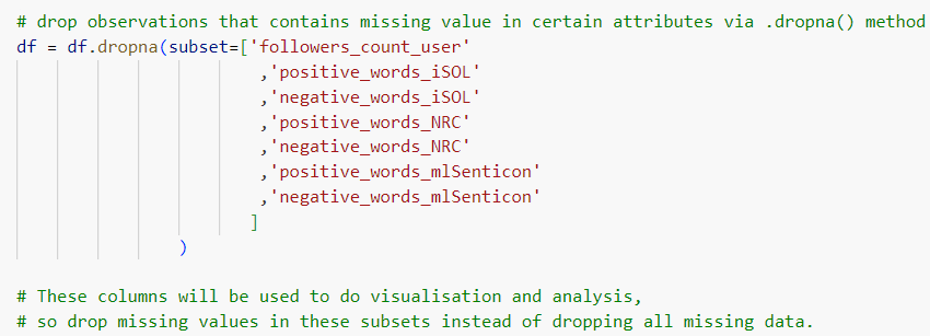
最初,仅通过 .dropna() 方法删除特定子集中的缺失值(图 4)。
然而,随后在使用 .astype() 方法修改数据类型时发生了错误(图 5)。
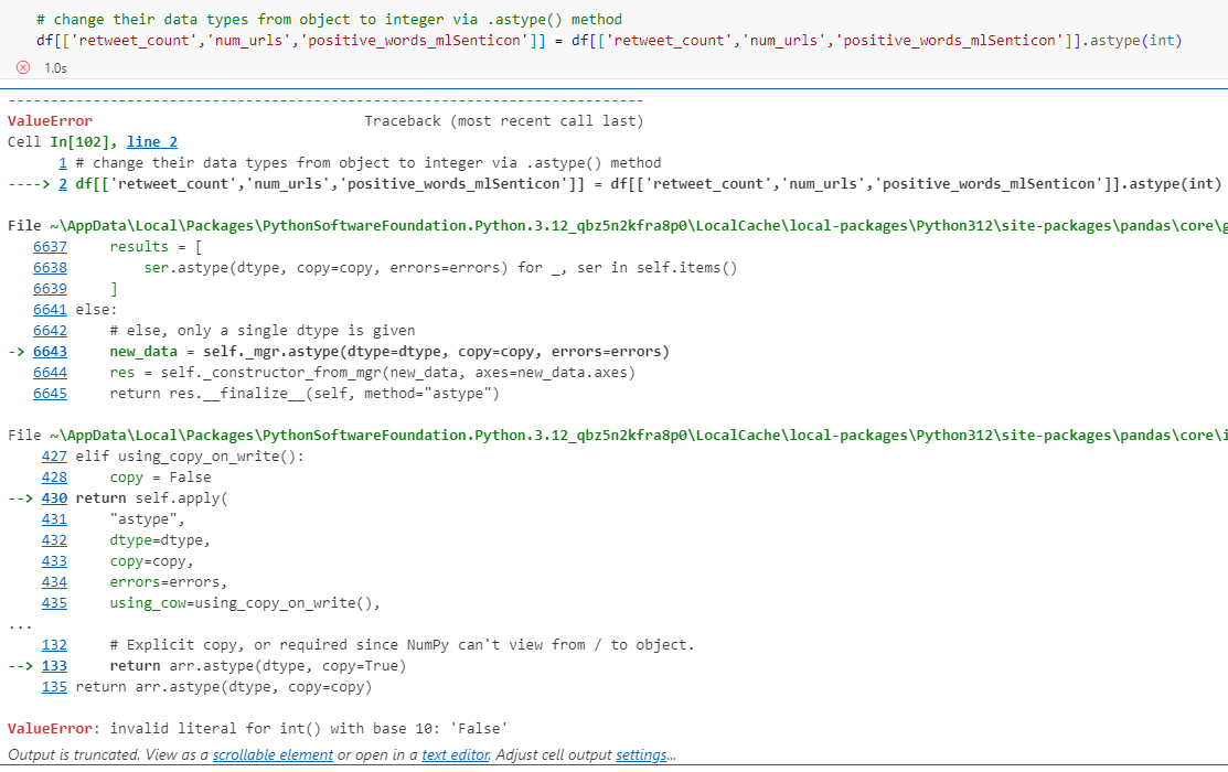
.astype(int) 时的报错
原因在于,这些属性中的字符串并非全部为数值型,因此无法直接通过 .astype(int) 转换为整数(图 6)。
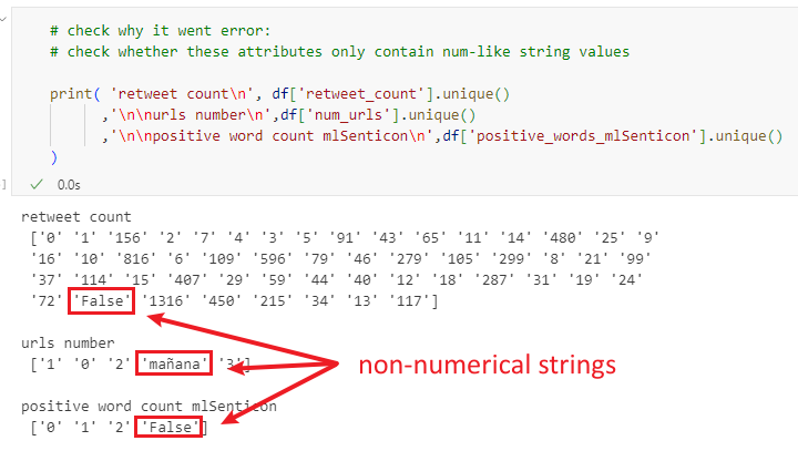
因此,在应用数据类型转换方法前,有必要先验证所有字符串是否均为数值型。此外发现,若在最初直接使用不带关键字参数的 .dropna() 删除所有缺失值,则不产生报错的概率将大幅提升。
图 3(作者受欢迎度直方图)通过 seaborn 的 .histplot() 函数绘制,并通过设置 hue 参数按颜色分组(图 7)。此方式会自动生成图例,以列名 ‘overall_sentiment’ 作为标题,但这并不适合作为图例标题。为此,尝试使用 plt.legend() 修改图例标题并保留其他信息,但效果不理想(如下图所示)。推测原因是 Seaborn 自动生成的图例与手动添加的 plt.legend() 之间存在冲突。
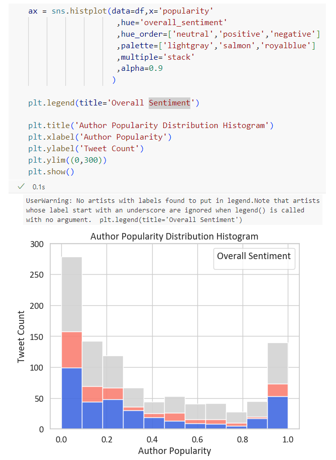
因此,将 plt.legend() 改为 ax.get_legend().set_title() ——该方法可检测当前图表中已生成的图例,并为其设置新标题。